2009 AMBER tutorial with Trpcage
For additional Rizzo Lab tutorials see AMBER Tutorials.
Contents
To Do
- explain outputs of md.in and min.in
- talk more about amber
- talk more about trpcage
About Amber
AMBER is a molecular dynamics program.
About Trp-cage
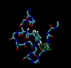
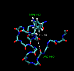
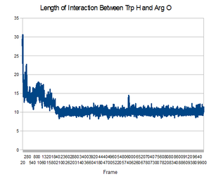
Trp-cage is a 20-residue miniprotein, which is believed to be the fastest folder known so far. One important characteristic of the folded structure is the hydrogen bond between the O from Arg and the H from Trp. It packs Trp, which is hydrophobic, inside the molecule.
Setting up parameters and initial coordinates with Leap/Getting Started
- MDtutorial_Amber10.pdf - the basic idea that we will follow, and render into this Wiki page
First move to your home directory and create a new directory for this project. (TrpCage)
cd .
mkdir TrpCage
In this tutorial, you will create a shell script. A shell script is a script that contains a series of commands that are executed in order. You will use this script to create the TrpCage protein and run in through the tleap program to create coordinate and topology files. First, create start the vi editor with a file called runleap.csh.
vi runleap.csh
With the file editor open, type in the following material.
#!/bin/csh
nice +10
hostname
date

set workdir = /home/rizzo/trp_cage_project #creating a directory to work on the tutorial. Change to the directory of you preference
mkdir -p $workdir
cd $workdir

echo "setpath for tleap"
set tleap = /opt/software/AMS536software/amber.ifort/exe/tleap
echo "Making tleap input"

cat << EOFA > trpcage.leap01.in
set default PBradii mbondi2
source leaprc.ff99
loadamberparams ~rizzo/public/parm.e16.dat  # you may want to copy this file to your own directory
trpcage = sequence {NASN LEU TYR ILE GLN TRP LEU LYS ASP GLY GLY PRO SER SER GLY ARG PRO PRO PRO CSER}
saveamberparm trpcage tc5b.top tc5b.crd
EOFA

echo "Running tleap"
$tleap -s -f trpcage.leap01.in > trpcage.leap01.out
An explanation of the following commands
- "#!/bin/csh" - necessary for a shell script to function
- nice +10 - runs the script at a lower priority to other jobs
- echo "text" - prints text in quotations - this helps indicate what jobs the script is performing
- set name = path - sets the path to the following the equals sign (double check this path on your machine by typing which tleap)
- cat << EOFA > trpcage.leap01.in - writes the following information to EOFA (end of file A) and outputs it to the file trpcage.leap01.in
- note the information following this line until EOFA contains the important information read by tleap.
- source leaprc.ff99 - references the parameters used to create protein
- trpcage = sequence {...} - names the amino acid series listed in the { } as trpcage; note the use of N preceding the ASN and C preceding the SER to indicate the nature of the terminuses of the sequence
- saveamberparm trpcage tc5b.top tc5b.crd - saves the topology of the trpcage sequence in a *.top file and the coordinates of the protein in the *.crd file
- $tleap -s -f trpcage.leap01.in > trpcage.leap01.out - executes the program tleap from the path name expressed above using the *.in file and outputs it to the *.out file (-s tells tleap to ignore the normal startup source and -f tells it to reference the trpcage.leap01.in)
Now we need to excute this csh file, what we should do is to use the command "csh filename".
csh runleap.csh
And then we got it excuted.
You now have created a number of useful files. Two which are particularly important are tc5b.crd and tc5b.top. You may use these to open your new protein in VMD. To do so, open a new session of VMD.
vmd
Here we entered VMD graphic interface.
1.Click "File->New Molecule"
2. Click "BROWSE" and select tc5b.top for the 0: tc5b.crd molecule. At the "Determine file type", select "AMBER7 Parm". Click "LOAD"
3. Click "BROWSE" and select tc5b.crd. At "Determine file type", select "AMBER7 Restart". then click "LOAD"
You now have your trpcage molecule loaded in VMD.
Preparing MD Simulation
After creating your .top and .crd files for your molecule, you should create the files read by sander for the minimization and the MD simulation.
The following is the input for the minimization, which will be called min.in:
 energy minimization
&cntrl
       ntx = 1,
       imin = 1, maxcyc=1000,
       saltcon = 0.0,
       igb=5, ntb = 0,
       ntwr = 100, ntpr = 100,
       scee = 1.2, cut = 99.0,
       nscm = 500,
&end
The input file for the MD simulation will be called md.in and has the following content:
 langevin dynamics simulation
&cntrl
       ntx = 1, irest=0,
       imin = 0, nstlim = 5000000, dt = 0.002,
       ntt = 3, gamma_ln=1., temp0 = 300.0, tempi=250.,
       ntc = 2, ntf = 2,
       igb=5, ntb = 0, saltcon = 0.0,
       ntwx = 500, ntwe = 0, ntwr = 500, ntpr = 500,
       scee = 1.2, cut = 99.0,
       nscm = 500,
&end
The parameters used in the min.in and md.in files are described below:
- ntx: initial coordinates, velocities and box size will be read from the input coordinates file, in this case, tc5b.crd. Value "1" is default and it means that the initial coordinates file will be read formatted with no initial velocity information. This option is usually used when one is starting from minimized or model-built coordinates, which is our case;
- imin: it is either "1" for an energy minimization or "0" for a molecular dynamics simulation;
- maxcyc: maximum number of cycles of minimization (default = 1);
- saltcon: sets the concentration (M) of 1-1 mobile counterions in solution, using a modified generalized Born based on limiting law for ion screening
of interactions;
- igb: defines which implicit solvent model will be used. Value "5" uses a modified GB model. With this option, it is necessary to "set default PBradii mbondi2", as we did in runleap.csh;
- ntb: specifies whether constant volume or constant pressure dynamics will be used for the periodic box. For value "0", a boundary will not applied regardless of any boundary condition information in the topology file;
- ntwr: at every NTWR steps, the result file (-r) will be written (updated);
- ntpr: at every NTPR steps energy information will be printed to the output file (-o) and information file (-inf);
- cut: specifies the nonbonded cutoff, in Angstroms;
- nscm: flag for the removal of translational and rotational center-of-mass (COM) motion at regular intervals;
- ntslim: number of steps of the simulation;
- dt: time step;
- irest: flag to restart the simualtion. Value "0" does not restart it;
- ntwx: at every NTWX steps the coordinates will be written to the trajectory coordinates file (-x).
- ntwe: at every NTWE steps the energies and temperatures will be written to the extensive file (-e);
- tempi: initial temperature;
- temp0: reference temperature at which the system is to be kept, if ntt>0;
- scee: 1-4 electrostatic interactions are divided by SCEE;
- gamma_ln: the collision frequency γ, in ps−1, when ntt = 3;
- ntt: switch for temperature scaling. Value "3" correspond to the canonical (constant T) ensemble;
- ntc: flag for SHAKE to perform bond length constraints. For value "1", SHAKE is not performed (default). For value "2", bonds involving hydrogen are constrained;
- ntf: force evaluation (necessary if SHAKE is used). For value "2", bond interactions involving H-atoms are omitted (used with NTC = 2);
From the dt and ntslim parameters you can have 10ns, which is how long the MD simulation will run.
Now you are ready to create the shell script to run your minimization and folding. To create the script, open a file in vi called run.sander:
vi run.sander
In the file, you will be creating a script to run an energy minimization and trajectory in succession. In the file, paste
#!/bin/csh
hostname
date
set workdir = "/home/pholden/amberproj/" #change it to the directory you are working on, where you ran tleap
cd $workdir

sander -O \
-i ./min.in \
-p ./tc5b.top \
-c ./tc5b.crd \
-o ./min.out \
-x ./min.x \
-e ./minex \
-v ./minvel \
-inf ./mininfo \
-r ./min.r

sander -O \
-i ./md.in \
-p ./tc5b.top \
-c ./min.r \
-o ./md.out \
-x ./md.x \
-e ./mden \
-v ./mdvel \
-inf ./mdinfo \
-r ./md.r
Notice from the file that we are running sander two times. The first run will perform energy minimization and the second run will perform the MD simulation. For both runs, there are many parameters set for sander. Below is a description of what each parameter means:
- -O: output files will be overwritten. Alternatively, one could use -A to append output files if they exist;
- -i: input file containing the characteristics of the run;
- -p: input file containing the molecular topology;
- -c: input file containing the initial coordinates of the molecule;
- -o: output file containing the energy and the temperature information at each ntpr steps;
- -x: output file containing the set of molecular coordinates obtained during trajectory. The coordinates are shown at each ntwx steps;
- -e: output file containing the extensive energy data saved during trajectory at each ntwe steps;
- -v: output file containing the set of velocities saved during trajectory. The velocities are shown at each ntwv steps;
- -inf: output file that shows the energy and the temperature information in the final step;
- -r: output file that contains the molecular coordinates in the final step.
To run the file, first open a secure shell in on the compute computer. To do so, type
ssh compute
Alternately if you are not in the mathlab when running sander, open a secure shell directly into compute.
Answer the questions until you receive a prompt.
Now that you are on the compute computer, type to execute your file.
csh run.sander &
By typing in & after the script name, it runs it in the background.
A note: The trpcage simulation will take at least one day running on the compute machine.
Looking at results
Type the command ls in you working directory. You will notice that many new files have been created. Some output files set for sander won't be created because they are not necessary in our simulation. For instance, there will be no mdvel file in you home directory since we started an MD simulation from a minimization.
First, you can look at the minimization exclusively. You may look at this while the trajectory is running the second time (something to do!).
Open a new VMD window. You must load the .top file before loading the coordinates for the minimization. To do so,
Load tc5b.top.  Select "AMBER7 Parm", as it is a parameter file.
Load min.r (in this case, this is a restart file).  Select "AMBER7 Restart" file.
You may wish to compare this to your initial molecule created by the tleap program. Load a new molecule with the tc5b.top and tc5b.crd files as instructed by the "Getting Started" section. They both should appear on your monitor. If you load the min.r as an additional restart file on top of this molecule (File --> load data into molecule --> select min.r as a "AMBER7 Restart" file) you now have one molecule with two frames.
As soon as your MD simulation finishes, you can look at how the structure changes during the trajectory. Open a new VMD window. You must load the .top file before loading the set of coordinates from the MD simulation. To do so,
Load tc5b.top.  Select "AMBER7 Parm", as it is a parameter file.
Load md.x.  Select "AMBER Coordinates" file.
Now, all of the structures obtained during the trajectory will be loaded. Each frame corresponds to the dt*ntwx*frame time of the simulation. The last frame has the final structure obtained from the MD simulation.
Simple Analyses
First let do an RMSD analysis to see how the simulation changes the struture of the molecular.
Quit VMD, and restart VMD by typing "VMD" into terminal
Load tc5b.top. Select "AMBER7 Parm", as it is a parameter file.
Load md.x, Select "AMBER Coordinates"
Now we loaded the simulated strucutre, and then we are going to load the original file.
Load tc5b.top. Select "AMBER7 Parm", as it is a parameter file.
Load tc5b.crd. Select "AMBER7 Restart", (Restart means it contains only one picture).
Now we have two strucutures in the screen. and We are going to do the RMSD in the next step.
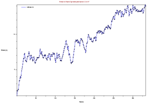
Now that you have your trajectory loaded in VMD, the first analysis you can do is to calculate the RMSD of the structure during the trajectory. Go to the VMD main menu and click on "Extensions->Analysis->RMSD Trajectory Tool". Click "Add all", Check the box "backbone" so that you only calculate the backbone RMSD (side chains will not be included in the calculation). Select the original strucutre id, Mark "Selected" Box, and Also check the box "Plot" so that you can see the graph. Now, click the "Align" button, and then click the "RMSD" button. You should have a plot like the shown below.
This image is from doing above with the md.x output file. Then file -> export to postscript. Then
pstoimg mdx.multiplot.ps mdx_multiplot.png
this produces an error, but also the .png file. My understanding is that this is showing the RMSD for every frame, compared to the first state. Looking at it in this light, the increasing RMSD is understandable, it is folding.
Notice how the structure changes during the simulation. Has the peptide already folded to the correct structure of trp-cage? To answer that, load the native structure in VMD. One can acquire the native structure of TrpCage by downloading the PDB file 1L2Y. To do so:
File --> New Molecule --> type 1L2Y --> click load molecule.
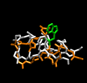
This file is a trajectory of 38 different acceptable frames of native structure. Any one of them is acceptable to compare your trajectory to. One can easily modify this pdb file so that it contains only one acceptable structure to compare it to. To do so, download the 1L2Y molecule from the pdb website. Copy the file first to have an unmodified original
cp 1L2Y.pdb 1L2Ymod.pdb
Open the copied pdb file in vi
vi 1L2Ymod.pdb
Modify the file by deleting the models after the first. You can search for ENDMDL
/ENDMDL
This will bring you to the end of the first MDL. You can delete to the end of the file except the last line (or perhaps including, I have to check).
Now you can load this modified pdb file into VMD. With your trajectory already loaded, click
File --> new molecule --> browse --> 1L2Ymod.pdb
It should automatically select pdb file. Click load. Now you have the native structure loaded for comparison to your simulation.
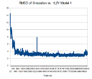
Having the native structure loaded, you can compare the last structure from the trajectory with the native structure. To have a better answer, you should compare the native structure to all of the structures in the trajectory. To do that, go back to the "RMSD Trajectory Tool". If both molecules are not listed, click the "Add All" button. Now, select the "Selected" box in the top right. This will let you select which molecule is the reference structure. The native structure will be the reference in this case, so click on it (it should be named 12LYmod.pdb). Don't forget to check the "Plot" box. Click the "Align" button and then the "RMSD" button.Note that this plot is a comparison of the positions of the backbone. It seems that relatively quickly the simulation approximates the native structure and then does not get any closer. This rmsd plot does not take into account sidechains.
From the plot, you can see which structure is closest to the native structure. How far is it from the native? Let us compare this structure to the native. You can know exactly in which frame this structure is by focusing your mouse in that point and then looking at the command window. The command window should show the structure x,y coordinates, in which x is the number of the frame. Now you can write the frame number in the left bottom of the VMD main menu. How alike are the structures?
Going Further
As a further analysis, the simulation can be run at alternate temperatures. To do so, a few simple changes need to take place first.
Create a new directory called trialtwo.
mkdir trialtwo
Copy the following files to the new directory: tc5b.top, run.sander, min.r, md.in.
For one of them: cp tc5b.top trialtwo/tc5b.top
Change the name of the run.sander so as not to confuse them when running it.
mv run.sander run1.sander
Modify the working directory in run.sander to ensure that the files created are in the new directory.
vi run.sander
Change the path for the "set workdir" command to the new directory created.
Delete the entire minimization section of the script.
The minimization should be the same as before and therefore does not need to be run again.
Modify the md.in to represent the new parameters for the new simulation.
vi md.in
Here, you can modify it as you wish. One possibility, discussed below, is running the simulation at a higher temperature to see if some of the folding barriers faced in the simulation at 300K could be overcome. Also, so the simulation could reveal the results sooner, the simulation was shorted to 5ns. In the md.in file, change the following parameters to:
nstlim = 2500000
temp0 = 350.0
Then, as before, run the shell script.
csh run.sander
Results of New Simulation
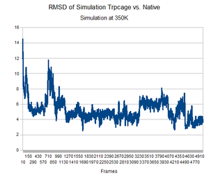
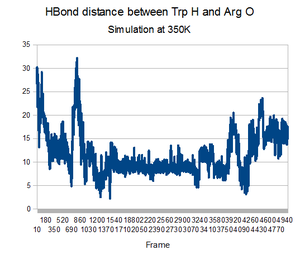
As predicted, the simulation at 350K allowed TrpCage to fold into new patterns. The analysis discussed before was performed on this new simulation. The RMSD analysis was performed, again comparing the backbone of the simulation to the backbone of the native state from the 1L2Y pdb file. Unsurprisingly, the results showed a greater variance and the simulation did not get to an equilibrium state as it did before.
Running the simulation at 350K for 550ns should produce the native structure. Further examinations of TrpCage at different temperatures could also produce the native state. Perhaps also running a simulated annealing of the protein would reproduce it as well.
Simulated Annealing
One might also be interested in furthering the examination of the folding of TrpCage by running a simulated annealing of the molecule. To begin this process, create a directory called annealing in your project directory.
mkdir annealing/
Copy the following files to that directory: tc5b.top, md.r, run.sander.
cp tc5b.top annealing/
cp md.r annealing/
Rename the run.sander file for clarity.
cp run.sander annealing/runanneal.sander
In the annealing directory, modify the new files runanneal.sander.
Modify the pathname to correspond to the new directory.
Delete the entire first sander run.
Change the -i file to be mdanneal.in
Change the -c file to be md.r
Modify the output files to have new unique names.  Try adding anneal to the name.
Create a new file in vi called mdanneal.in
vi mdanneal.in
In the file, copy the following text. This file contains the parameters for the sander run.
langevin dynamics simulations
 &cntrl
        ntx = 1, irest=0,
        imin = 0, nstlim = 4500000, dt = 0.002,
        ntt = 3, gamma_ln=1., temp0 = 300.0, tempi=200.,
        ntc = 2, ntf = 2,
        igb=5, ntb = 0, saltcon=0.,
        ntwx = 500, ntwe = 0, ntwr = 500, ntpr = 500,
        scee = 1.2, cut = 100.0,
        nscm = 500, nmropt = 1,
 /
 &wt type='TEMP0', istep1=0,istep2=500000,
   value1=300.0, value2=400.0
 /
 &wt type='TEMP0', istep1=500001,istep2=1500000,
   value1=400.0, value2=400.0
 /
 &wt type='TEMP0', istep1=1500001,istep2=2500000,
   value1=400.0, value2=350.0
 /
 &wt type='TEMP0', istep1=2500001,istep2=3500000,
   value1=350.0, value2=300.0
 /
 &wt type='TEMP0', istep1=3500001,istep2=4500000,
   value1=300.0, value2=300.0
 /
 &wt type='END'
 /
The contents of this file are slightly different from the original md.in file you wrote. Most notably:
- nmropt = 1 - this indicates you will be modifying weights (in this case temperature) throughout the simulation
- &wt - indicates in the new weight change
- type='TEMP0' - indicates a change in the temperature of our system
- istep1=x, istep2=y - indicates which range of steps the change will take place on
- value1=x, value2=y - indicates which Temps (in this case) you will be changing from (x) and to (y) over the course of the indicated range of steps; note if x=y in this case, no temperature is changing during these time steps.
- &wt type='END' - you must end the changes in weights with this command
- ntwe = 0 - you may wish to change this to 500 so you can have energy and temperature outputs for each frame
By using the md.r file as the original coordinate file, you will be taking advantage of the 10ns of equilibration you've already done at 300K. This is why this script starts with a dramatic increase in temperature as opposed to steps of equilibration. Note the original minimization was also left out of the runanneal.sander script because the minimization already took place in the original equilibration.
Results
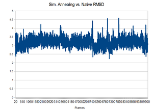
Unfortunately, the equilibrated state produced by the 300K initial equilibration seemed to produce a quite stable structure. During the higher temperatures of the annealing process, no dramatic change to the backbone occurred. It would not have been able to make a change because it did not have enough energy to overcome the favorable interactions that existed in the pocket. This is shown by the lack of change in the backbone RMSD compared to the native state.Perhaps higher temperatures might be in order.
