Difference between revisions of "2024 DOCK tutorial 1 with PDBID 2ITO"
Stonybrook (talk | contribs) (→Fixed Anchor Docking) |
Stonybrook (talk | contribs) (→Generating the Grid) |
||
| (2 intermediate revisions by the same user not shown) | |||
| Line 174: | Line 174: | ||
#Close any open sessions in Chimera | #Close any open sessions in Chimera | ||
#In Chimera open selected_spheres.sph | #In Chimera open selected_spheres.sph | ||
| − | #In the current session, open the original protein/ligand complex ( | + | #In the current session, open the original protein/ligand complex (2ito.pdb) |
#Observe the spheres located within the binding site of the protein, similar to: | #Observe the spheres located within the binding site of the protein, similar to: | ||
| Line 235: | Line 235: | ||
distance_dielectric yes | distance_dielectric yes | ||
dielectric_factor 4 | dielectric_factor 4 | ||
| − | |||
bump_filter yes | bump_filter yes | ||
bump_overlap 0.75 | bump_overlap 0.75 | ||
| Line 624: | Line 623: | ||
The steps for the next docking mode should also be similar. | The steps for the next docking mode should also be similar. | ||
| − | === | + | ===Flexible Docking=== |
In this session, we will be showing the tutorial for Flexible Docking. Among the three docking methods introduced in this tutorial, this would be the most computationally expensive method since the algorithm will be sampling all of the possible conformations of each input ligand and test their binding ability with the binding site. Thus, one might expect the computing time for this method to be exceed other introduced methods. | In this session, we will be showing the tutorial for Flexible Docking. Among the three docking methods introduced in this tutorial, this would be the most computationally expensive method since the algorithm will be sampling all of the possible conformations of each input ligand and test their binding ability with the binding site. Thus, one might expect the computing time for this method to be exceed other introduced methods. | ||
Latest revision as of 01:15, 17 April 2024
Contents
- 1 Introduction
- 2 Preparation of the ligand and protein
- 3 Creating the Protein Binding Site Surface
- 4 Box and Grid Generation
- 5 Energy Minimization
- 6 DOCK
- 7 Virtual Screening of a Ligand Library
- 8 Cartesian Minimization of Virtually Screened Small Molecules
- 9 Rescoring and Ranking Virtually Screened Molecules
Introduction
When the function of a protein gets involved in multiple diseases, it becomes a target protein. Pharmaceutical companies target this protein by developing small-molecule inhibitors to prevent its function. Earlier scientists used to identify these molecules by High Throughput Screening where these small molecules would be chemically synthesized and exposed to cells to determine their activity. This method was time-consuming and expensive to employ. When Virtual Screening came into the market it eased the whole process of screening the activity of thousands of molecules using computational algorithms.
A virtual screen is set up by preparing the structure of the receptor by adding appropriate charges and hydrogens, which is also done for the ligand that we want to dock the receptor to. A footprint is then generated to identify the receptor residues where the ligand can bind. A molecular modeling program named DOCK is used here to dock our protein of interest with ligand.
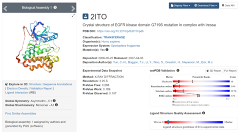
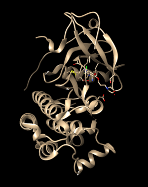
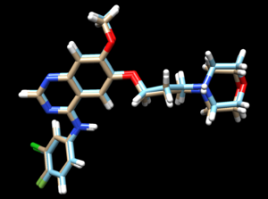
DOCK employs algorithms to bring together the ligand and the receptor together. This tutorial would involve preparing a protein and ligand for docking by downloading a protein-ligand complex from RCSB PDB database (https://www.rcsb.org/), which in this tutorial is 2ITO, which is a crystal structure of G719S mutation in EGFR Kinase domain, in complex with Iressa (an EGFR inhibitor)
These website tutorials are useful if you are unfamiliar with the following tools:
This tutorial is for PDBID 2ITO. Replace any reference to 2ITO with the protein of your choice.
Learning Objectives
- Download Protein of interest from RCSB PDB database
- Step-by-step guide to use DOCK6.10 for docking protein of interest with a small-molecule ligand
- Analyse docking results to identify the most favorable binding geometry between the protein and ligand
Setting Up Your Environment
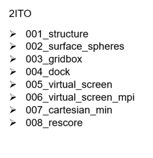
Before beginning the docking process, the following directory structure should be set up in the seawulf cluster under the desginated group name:
Downloading a protein from the PDB database
Download a protein complex from RCSB PDB database. As part of this tutorial, the complex 2ITO will be used. On the main page, to the right of the top, there will be a search bar in which you will type in the PDBID and press Enter.
The resulting protein complex would be in display.
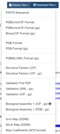
Towards the right hand side, click on Download Files, and select "Biological Assembly 1 (PDB - gz)"
The file will be saved in the local directory.
Preparation of the ligand and protein
The following steps would demonstrate the preparation of the protein and the ligand which would be used by DOCK6.10. The steps in this section will be performed using Chimera. These steps are essential to perform so as to ensure accurate analysis of the data post the docking step. This section will demonstrate:
- Evaluating the structure to determine any missing loops
- Adding Missing Loops using Modeller
- Prepare the protein structure
- Prepare the ligand structure
Evaluating the Structure
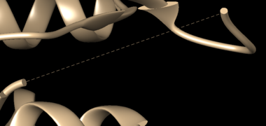
Use Chimera to open the downloaded PDB structure. While visualizing the structure in Chimera, note for any missing loops present, which is indicated by dashed lines in the structure.
To fix the missing sections, go to Tools → Surface Editing → Model/Refine Loops. Two dialogue boxes will appear:
this box shows the sequence of amino acids in the PDB structure.
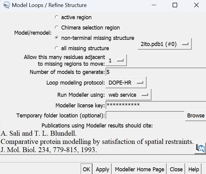
The second box has the required inputs to give Chimera so it can re-model the missing loops:
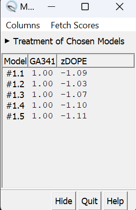
in this box choose 'non-terminal missing structure' and click 'Apply'. The progress of Modeller can be monitored in the lower left hand corner of the display. Once it has finished, another dialogue box will appear showing the five choices of models for the missing sections.
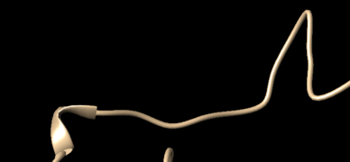
When clicking on each of the results, the fixed missing section will show up. Decide which one you want to keep, highlight it and save the file by choosing File → Save PDB. In the dialogue box, be sure to give this file a new name so as not to overwrite the original 2ito.pdb file, something similar to 2ito_loops_fixed.pdb. In the 'Save models' section, choose the model number chosen. To confirm that everything has worked correctly, close the current session in Chimera and open 2ito_loops_fixed.pdb. Now no dashed lines should be seen and only the structure with the fixed loops.
Preparing the Protein file
The first step in preparing the protein is to get the protein structure alone in a .pdb file. To do this:
- Select an atom on the protein
- Press the up arrow until the entire protein is selected
- Go to Select → Invert (all models). This will change the selection from the protein to everything else in the structure
- Go to Actions → Atoms/Bonds → Delete
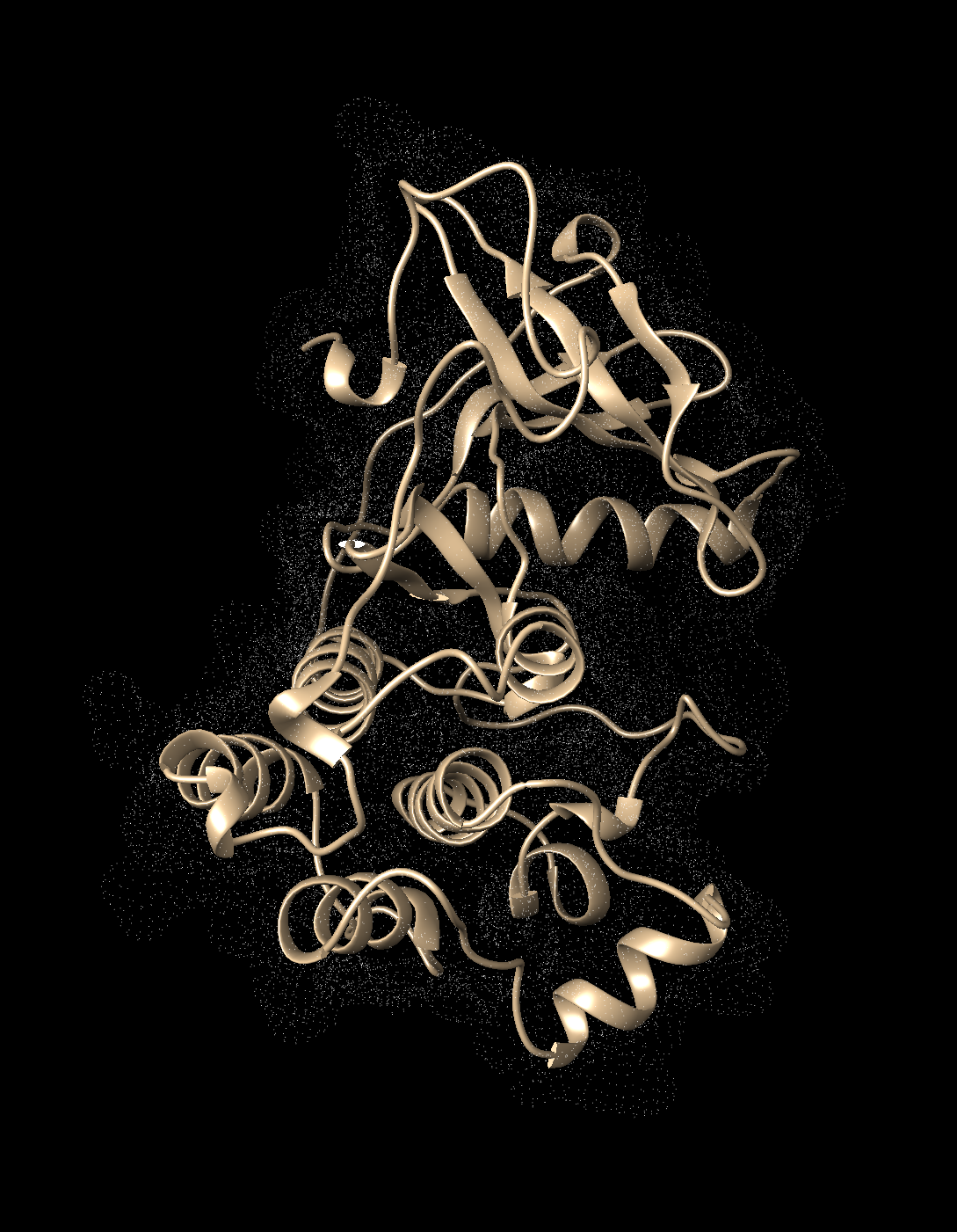
- Save the structure with a new file name (i.e. 2ito_protein_only.pdb). Your pdb file will now look similar to this:
At this point we also need to generate a .mol2 file for the structure in this state. Go to File → Save Mol2 and give the file a descriptive name such as 2ito_protein_no_hydrogens_no_charges.mol2
There are now two more steps necessary for its preparation:
- Adding hydrogens
- Adding charge
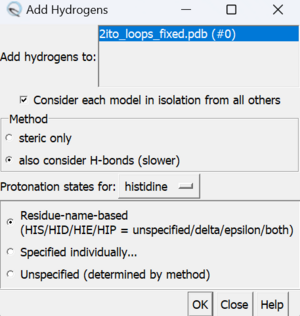
To add hydrogen atoms click on: Tools → Structure Editing → AddH. This command will cause the following dialogue box to appear:
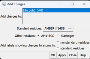
If the hydrogen atoms were successfully added, white ends to the atoms would appear which are the hydrogens. The final step is to add charges to the protein. To add charges click on Tools → Structure Editing → Add Charge and the following dialogue box will show up:
Click on 'OK' and once the program is finished the bottom left hand corner tells what the total charge of the structure is. This number should be an integer. The protein structure is now completely prepared and ready for docking. The final step is to save two files, a .pdb of the structure in this state and a .mol2 file. Simply go to File → Save PDB and choose a filename such as 2ito_charges.pdb; then go to File → Save Mol2 and choose a filename such as 2ito_protein_with_charges.mol2.
Preparing the Ligand File
The first step in preparing the ligand is the same as for the protein - to get the ligand structure alone in a .pdb file. To do this:
- Select an atom on the ligand
- Press the up arrow until the entire ligand is selected (press the up arrow many times)
- Go to Select → Invert (all models). This will change the selection from the ligand to everything else in the structure
- Go to Actions → Atom/Bonds → Delete
Before we start preparing the ligand for docking we need to again save a .mol2 file for the structure in this state. Go to File → Save Mol2 and give the file a descriptive name such as 2ito_no_hydrogens_no_charges.mol2
Once the ligand is saved as its own file the same two steps are followed as for the protein:
- Add hydrogens
- Add charges
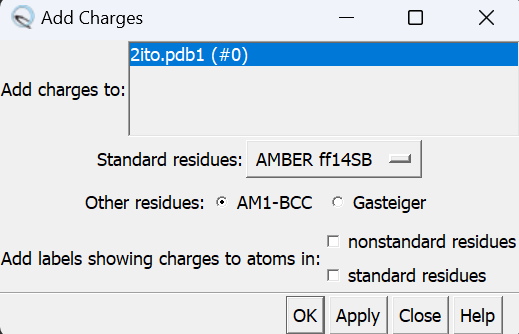
The final step is to add charges to the ligand. The same steps as for the protein are followed except after the dialogue box appear and click 'OK', a second box will appear:
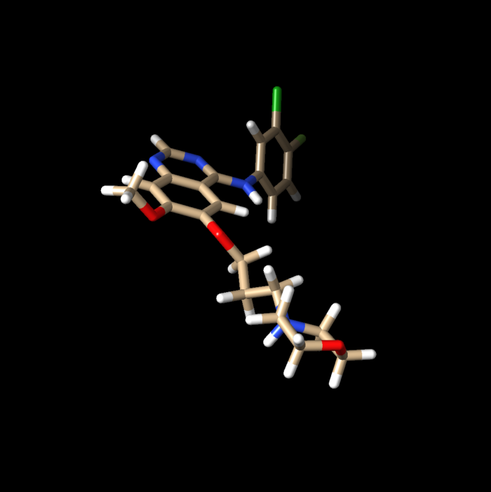
When the program is completed, the total charge calculated for the ligand in the lower left hand corner. This number should be an integer (or close to it).
The ligand is ready for docking.
The final step is to again save two files, a .pdb and .mol2 of the structure in this state. Go to File → Save Mol2 and give the file a name such as 2ito_ligand_hydrogens_charges.mol2 and File → Save PDB and give the file a name such as 2ito_ligand_hydrogens_charges.pdb.
- Save the structure with a new file name (i.e. 2ito_ligand_only.pdb).
Final Steps
Before moving onto finding the binding site of the protein move the four .mol2 files over to Seawulf. Do this using the following scp command:
scp *.mol2 username@login.seawulf.stonybrook.edu:'/gpfs/projects/AMS536/YOURYEAR/students/YOURGROUP/001_structure'
Creating the Protein Binding Site Surface
This section walks through the steps necessary to identify the binding site of the protein using a function within DOCK to place surface spheres along the protein.
Creating the Required Surface (DMS) File
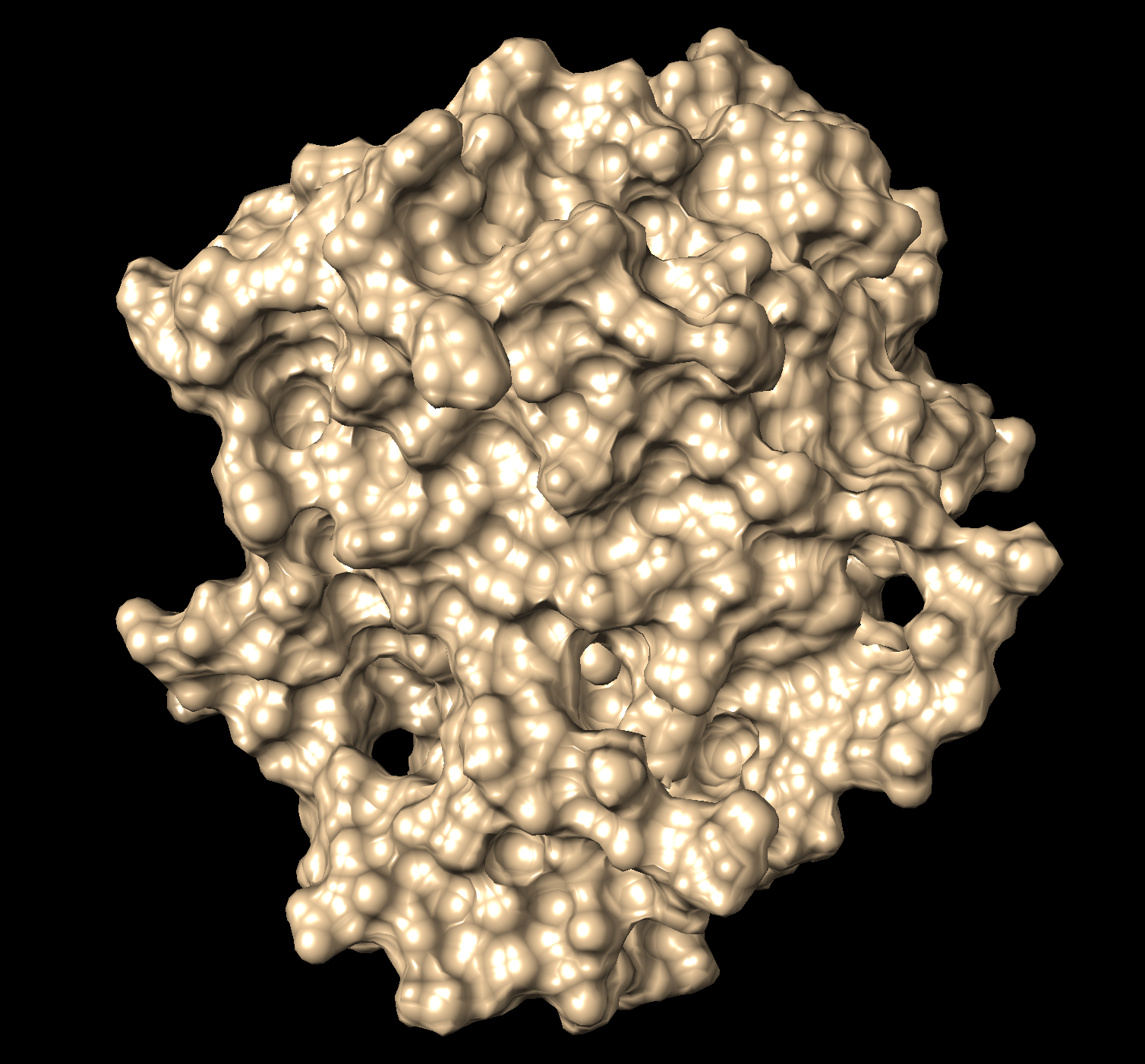
In Chimera, open the 2ito_protein_only.pdb file. Go to Actions → Surface → show. This will display the van der Waals surface of the protein. The image should be similar to:
Once this is done the .dms file needs to be generated by clicking on Tools → Structure Editing → Write DMS. A dialogue box will appear the file will be given a name, such as 2ito_surface.dms. Once this file is saved, make sure that nothing unintended happened with DOCK during its generation. This is done by overlaying the .dms file with the protein_only file. To do this, close current session, open the 2ito_protein_only.pdb and then open the 2ito_surface.dms. If everything worked as it should an image should be seen similar to:
The small dots (which is the .dms file) is perfectly aligned over the protein structure. Now that it's verified that everything looks good, further steps can be continued.
Generating Spheres for the Binding Site
Now that a .dms file has been generated, the binding site of the protein is found using a DOCK program called sphgen. This program is run on the command line on Seawulf. In order for it to run properly one needs to scp the .dms file to the 002_surface_spheres directory using the command:
scp filename.dms username@login.seawulf.stonybrook.edu:'/gpfs/projects/AMS536/YOURYEAR/students/YOURGROUP/002_surface_spheres'
Once the file is in the 002_surface_spheres directory to create a file to run sphgen. Type:
vi INSPH
this will open a new text document with the name INSPH. Put the following in the document replacing the filenames with your specific files:
 2ito_surface.dms
 R
 X
 0.0
 4.0
 1.4
 2ito.sph
Note that the first and last lines need to be updated to be the name of the protein files. Save this file and return to the command line using the command:
sphgen -i INSPH -o OUTSPH
When this is completed you will see the 2ito.sph in the directory. Once again one needs to verify that this file was generated properly. Do this by comparing it to the original .pdb. Using scp, move the output file (in this case 2ito.sph) back to your local computer and open the file in a new Chimera session. In the same session, open the original .pdb file and the two structures should be aligned to each other. The image should be similar to:
As one could see, the ribbon of the original file is aligned to the spheres just generated. At this point one can move onto the next step of selecting the spheres within the binding site of the protein.
Binding Site Spheres
This step runs a DOCK program called sphere_selector which is again run on the command line. Log back in to Seawulf and move to your 002_surface_spheres directory. Then type:
sphere_selector 2ito.sph ../001_structure/2ito_ligand_hydrogens_charges.mol2 10.0
When this program has successfully completed and a new file will be seen in the directory called selected_spheres.sph. This file generated spheres which should line up with the binding site of the protein. To verify this in Chimera:
- scp selected_spheres.sph to local computer
- Close any open sessions in Chimera
- In Chimera open selected_spheres.sph
- In the current session, open the original protein/ligand complex (2ito.pdb)
- Observe the spheres located within the binding site of the protein, similar to:
While this looks good one should verify that the spheres are actually where the ligand is. This is done by selecting the spheres, hiding them from view, and verifying the ligand is in the same location:
- Hold down ctrl and click on a sphere
- Press the up arrow until all spheres are selected
- Actions → Atoms/Bonds → hide
- Verify the ligand is where the spheres were
as it can be seen the ligand is where the spheres were so one can be confident in their work so far.
Box and Grid Generation
The next step in the docking process is the box and grid generation. Instead of generating the energy interactions between all atoms of the protein and ligand, DOCK gets around this computationally expensive step by focusing solely on the area of interest around the protein-ligand binding pocket. Atoms that are far away from this site can be thought to have negligible impact on the energy interactions.
Generating the Box
The first step is to create a box around the active site. Create a DOCK program called showbox. Do this in the 003.gridbox directory.
vi showbox.in
This creates a new file called showbox.in and open it in vi. You will then need to type the following in the file:
 Y
 8.0
 ../002.surface_spheres/selected_spheres.sph
 1
 2ITO.box.pdb
This will automoatically construct boxes to enclose the spheres, give 8.0 Angstroms from the spheres to draw the box, tells the file where to find the sphere file that we had previously generated, the cluster number, and the output filename.
To run this file, type the following to receive 2ITO.box.pdb in your directory
showbox < showbox.in
After running this script, 2ITO.box.pdb should show up in your directory.
Generating the Grid
The next step is to generate the grid. Create a DOCK program called grid.
vi grid.in
Use the following code:
 allow_non_integral_charges                no
 compute_grids                             yes
 grid_spacing                              0.4
 output_molecule                           no
 contact_score                             no
 energy_score                              yes
 energy_cutoff_distance                    9999
 atom_model                                a
 attractive_exponent                       6
 repulsive_exponent                        9
 distance_dielectric                       yes
 dielectric_factor                         4
 bump_filter                               yes
 bump_overlap                              0.75
 receptor_file                             ../001.structure/2ITO_protein_rec_final.mol2
 box_file                                  2ITO.box.pdb
 vdw_definition_file                       /gpfs/projects/AMS536/zzz.programs/dock6.10/parameters/vdw_AMBER_parm99.defn
 score_grid_prefix                         grid
Once this file is saved, run it with the following code:
grid -i grid.in -o 2ITOGridInfo.out
This will take a while to run and after it finishes, you should have the following in your repository:
- grid.bmp
- grid.nrg
- 2ITOGridInfo.out
Energy Minimization
To allow DOCK to accurately calculate the energy interactions between atoms of the protein and ligand, it is important to make sure the ligand is in the lowest energy state before docking it into the binding site of the protein.
Ligand Minimization
Move on to the 004.energy_min directory. Create a DOCK program called min:
vi min.in
Use the following code:
 conformer_search_type                                        rigid
 use_internal_energy                                          yes
 internal_energy_rep_exp                                      12
 internal_energy_cutoff                                       100.0
 ligand_atom_file                                             ../001.structure/2ITO_ligand_Gefitinib_final.mol2
 limit_max_ligands                                            no
 skip_molecule                                                no
 read_mol_solvation                                           no
 calculate_rmsd                                               yes
 use_rmsd_reference_mol                                       yes
 rmsd_reference_filename                                      ../001.structure/2ITO_ligand_Gefitinib_final.mol2
 use_database_filter                                          no
 orient_ligand                                                no
 bump_filter                                                  no
 score_molecules                                              yes
 contact_score_primary                                        no
 contact_score_secondary                                      no
 grid_score_primary                                           yes
 grid_score_secondary                                         no
 grid_score_rep_rad_scale                                     1
 grid_score_vdw_scale                                         1
 grid_score_es_scale                                          1
 grid_score_grid_prefix                                       ../003.gridbox/grid
 multigrid_score_secondary                                    no
 dock3.5_score_secondary                                      no
 continuous_score_secondary                                   no
 footprint_similarity_score_secondary                         no
 pharmacophore_score_secondary                                no
 descriptor_score_secondary                                   no
 gbsa_zou_score_secondary                                     no
 gbsa_hawkins_score_secondary                                 no
 SASA_score_secondary                                         no
 amber_score_secondary                                        no
 minimize_ligand                                              yes
 simplex_max_iterations                                       1000
 simplex_tors_premin_iterations                               0
 simplex_max_cycles                                           1
 simplex_score_converge                                       0.1
 simplex_cycle_converge                                       1.0
 simplex_trans_step                                           1.0
 simplex_rot_step                                             0.1
 simplex_tors_step                                            10.0
 simplex_random_seed                                          0
 simplex_restraint_min                                        yes
 simplex_coefficient_restraint                                10.0
 atom_model                                                   all
 vdw_defn_file                                                /gpfs/projects/AMS536/zzz.programs/dock6.10/parameters/vdw_AMBER_parm99.defn
 flex_defn_file                                               /gpfs/projects/AMS536/zzz.programs/dock6.10/parameters/flex.defn
 flex_drive_file                                              /gpfs/projects/AMS536/zzz.programs/dock6.10/parameters/flex_drive.tbl
 ligand_outfile_prefix                                        2ITO.lig.min
 write_orientations                                           no
 num_scored_conformers                                        1
 rank_ligands                                                 no
Run with the following:
dock6 -i min.in -o min.out
2 new files will be outputted to your directory:
- min.out
- 2ITO.lig.min.mol2
The mol2 file should look like this:
The 2ITO.ligand from PDB with hydrogen and charges is brown and the newly generated 2ITO.lig.min.mol2 is blue.
Footprint Analysis
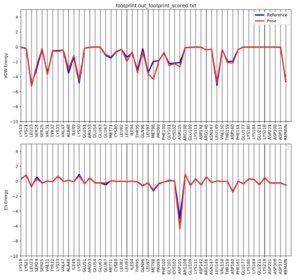
Footprint analysis allows us to visualize the electrostatic and VDW interactions between the ligand and protein. This is useful when designing new ligands to compare the set of energetics.
In the 005.footprint directory, create a DOCK program called footprint.
vi footprint.in
Use the following code:
 conformer_search_type                                        rigid
 use_internal_energy                                          no
 ligand_atom_file                                             2ITO.lig.min_scored.mol2
 limit_max_ligands                                            no
 skip_molecule                                                no
 read_mol_solvation                                           no
 calculate_rmsd                                               no
 use_database_filter                                          no
 orient_ligand                                                no
 bump_filter                                                  no
 score_molecules                                              yes
 contact_score_primary                                        no
 contact_score_secondary                                      no
 grid_score_primary                                           no
 grid_score_secondary                                         no
 multigrid_score_primary                                      no
 multigrid_score_secondary                                    no
 dock3.5_score_primary                                        no
 dock3.5_score_secondary                                      no
 continuous_score_primary                                     no
 continuous_score_secondary                                   no
 footprint_similarity_score_primary                           yes
 footprint_similarity_score_secondary                         no
 fps_score_use_footprint_reference_mol2                       yes
 fps_score_footprint_reference_mol2_filename                  ../001.structure/2ITO_ligand_Gefitinib_final.mol2
 fps_score_foot_compare_type                                  Euclidean
 fps_score_normalize_foot                                     no
 fps_score_foot_comp_all_residue                              yes
 fps_score_receptor_filename                                  ../001.structure/2ITO_protein_rec_final.mol2
 fps_score_vdw_att_exp                                        6
 fps_score_vdw_rep_exp                                        9
 fps_score_vdw_rep_rad_scale                                  1
 fps_score_use_distance_dependent_dielectric                  yes
 fps_score_dielectric                                         4.0
 fps_score_vdw_fp_scale                                       1
 fps_score_es_fp_scale                                        1
 fps_score_hb_fp_scale                                        0
 pharmacophore_score_secondary                                no
 descriptor_score_secondary                                   no
 gbsa_zou_score_secondary                                     no
 gbsa_hawkins_score_secondary                                 no
 SASA_score_secondary                                         no
 amber_score_secondary                                        no
 minimize_ligand                                              no
 atom_model                                                   all
 vdw_defn_file                                                /gpfs/projects/AMS536/zzz.programs/dock6.10/parameters/vdw_AMBER_parm99.defn
 flex_defn_file                                               /gpfs/projects/AMS536/zzz.programs/dock6.10/parameters/flex.defn
 flex_drive_file                                              /gpfs/projects/AMS536/zzz.programs/dock6.10/parameters/flex_drive.tbl
 ligand_outfile_prefix                                        footprint.out
 write_footprints                                             yes
 write_hbonds                                                 yes
 write_orientations                                           no
 num_scored_conformers                                        1
 rank_ligands                                                 no
Run the following to generate the footprint:
dock6 -i footprint.in
3 files will be added to this inventory
- 2ITO_footprint.out_footprint_scored.txt
- 2ITO_footprint.out_hbond_scored.txt
- 2ITO_footprint.out_scored.mol2
Now we need to visualize the results with a python script. Copy it from the class directory to your 005.footprint directory with the following:
cp /gpfs/projects/AMS536/zzz.programs/plot_footprint_single_magnitude.py .
Load up python with the following:
module load py/2.7.15
Then run the script with the following:
python plot_footprint_single_magnitude.py 2ITO_footprint.out_footprint_scored.txt 50
Once this script is complete, footprint.out_footprint_scored.txt.pdf should show up in your directory. Copy it onto your local computer to open it up. The file should look like this:
DOCK
There are 3 types of docking that we will be covering in this tutorial. The types and key differences are displayed below:
- Rigid Docking - conformation search: rigid, orient: yes
- Fixed Anchor Docking - conformation search: flex, orient: no
- Flexible Docking - conformation search: flex, orient: yes
Rigid Docking
Rigid docking treats the ligand as a rigid structure and fits it the best it can into the binding site of the protein. We will be working in the 006.rigid_docking directory.
Create the rigid.in file using the command:
vi rigid.in
The following lines need to be typed into the file:
 conformer_search_type                                        rigid
 use_internal_energy                                          yes
 internal_energy_rep_exp                                      12
 internal_energy_cutoff                                       100.0
 ligand_atom_file                                             2ITO.lig.min_scored.mol2
 limit_max_ligands                                            no
 skip_molecule                                                no
 read_mol_solvation                                           no
 calculate_rmsd                                               yes
 use_rmsd_reference_mol                                       yes
 rmsd_reference_filename                                      2ITO.lig.min_scored.mol2
 use_database_filter                                          no
 orient_ligand                                                yes
 automated_matching                                           yes
 receptor_site_file                                           ../002.surface_spheres/selected_spheres.sph
 max_orientations                                             1000
 critical_points                                              no
 chemical_matching                                            no
 use_ligand_spheres                                           no
 bump_filter                                                  no
 score_molecules                                              yes
 contact_score_primary                                        no
 contact_score_secondary                                      no
 grid_score_primary                                           yes
 grid_score_secondary                                         no
 grid_score_rep_rad_scale                                     1
 grid_score_vdw_scale                                         1
 grid_score_es_scale                                          1
 grid_score_grid_prefix                                       ../003.gridbox/grid
 multigrid_score_secondary                                    no
 dock3.5_score_secondary                                      no
 continuous_score_secondary                                   no
 footprint_similarity_score_secondary                         no
 pharmacophore_score_secondary                                no
 descriptor_score_secondary                                   no
 gbsa_zou_score_secondary                                     no
 gbsa_hawkins_score_secondary                                 no
 SASA_score_secondary                                         no
 amber_score_secondary                                        no
 minimize_ligand                                              yes
 simplex_max_iterations                                       1000
 simplex_tors_premin_iterations                               0
 simplex_max_cycles                                           1
 simplex_score_converge                                       0.1
 simplex_cycle_converge                                       1.0
 simplex_trans_step                                           1.0
 simplex_rot_step                                             0.1
 simplex_tors_step                                            10.0
 simplex_random_seed                                          0
 simplex_restraint_min                                        no
 atom_model                                                   all
 vdw_defn_file                                                /gpfs/projects/AMS536/zzz.programs/dock6.10/parameters/vdw_AMBER_parm99.defn
 flex_defn_file                                               /gpfs/projects/AMS536/zzz.programs/dock6.10/parameters/flex.defn
 flex_drive_file                                              /gpfs/projects/AMS536/zzz.programs/dock6.10/parameters/flex_drive.tbl
 ligand_outfile_prefix                                        rigid.out
 write_orientations                                           no
 num_scored_conformers                                        1
 rank_ligands                                                 no
This will take a few minutes to complete but once it is done, you should see the following files in your directory.
- rigid.out_scored.mol2
- rigid.out
Move the .mol2 file to your local computer and visualize it in Chimera. Compare it with the lig.min_scored,mol2 and you should see the following:
The 2ITO.lig.min_scored.mol2 is blue and the newly generated fixed.out_scored.mol2 is brown.
Look at the rigid.out file. This will allow you to look at the scoring:
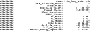
 Molecule: 2ito.pdb1
 Elapsed time for docking:      26 seconds
 Anchors:               1
 Orientations:          1000
 Conformations:         992
                         Grid_Score:          -72.913971
                    Grid_vdw_energy:          -63.204918
                     Grid_es_energy:           -9.709055
          Internal_energy_repulsive:           11.595561
 1 Molecules Processed
Fixed Anchor Docking
In this session, we will be showing the tutorial for Fixed Anchor Docking. For this mode of docking, the algorithm would first identify the largest fragment extracted from original ligand input. Noted that, the fragments are segmented based on the rotatable bonds of the ligands. Starting from this fragment pose, the algorithm will use it as an anchor to continuously add segments until the whole original ligand pose has been fully re-grown. Noted that when each fragment is added, it would be oriented for a pose that is energetically minimal. Comparing this method to the previous rigid docking mode, fixed anchor docking offer flexibility to the side chain while still being able to keep the general location of the ligand’s binding site as it fixes the anchor position.
Please navigate to the directory designated for this docking mode: 007.fixed_anchor_docking. Here, we can start create the input parameters, file name – fixed.in:
vi fixed.in
The following is the input parameter for fixed anchor docking. While you can copy and paste this into the body of your script, please make sure to change the input files directory (ligand and protein structure folder) to your personal directory. Also it should be a good practice to make sure the directories for the dock parameters should also be up-to-date.
 conformer_search_type                                        flex
 write_fragment_libraries                                     no
 user_specified_anchor                                        no
 limit_max_anchors                                            no
 min_anchor_size                                              5
 pruning_use_clustering                                       yes
 pruning_max_orients                                          1000
 pruning_clustering_cutoff                                    100
 pruning_conformer_score_cutoff                               100.0
 pruning_conformer_score_scaling_factor                       1.0
 use_clash_overlap                                            no
 write_growth_tree                                            no
 use_internal_energy                                          yes
 internal_energy_rep_exp                                      12
 internal_energy_cutoff                                       100.0
 ligand_atom_file                                             ../004.energy_min/2tio.lig.min_scored.mol2
 limit_max_ligands                                            no
 skip_molecule                                                no
 read_mol_solvation                                           no
 calculate_rmsd                                               yes
 use_rmsd_reference_mol                                       yes
 rmsd_reference_filename                                      ../004.energy_min/2tio.lig.min_scored.mol2
 use_database_filter                                          no
 orient_ligand                                                no
 bump_filter                                                  no
 score_molecules                                              yes
 contact_score_primary                                        no
 contact_score_secondary                                      no
 grid_score_primary                                           yes
 grid_score_secondary                                         no
 grid_score_rep_rad_scale                                     1
 grid_score_vdw_scale                                         1
 grid_score_es_scale                                          1
 grid_score_grid_prefix                                       ../003.gridbox/grid
 multigrid_score_secondary                                    no
 dock3.5_score_secondary                                      no
 continuous_score_secondary                                   no
 footprint_similarity_score_secondary                         no
 pharmacophore_score_secondary                                no
 descriptor_score_secondary                                   no
 gbsa_zou_score_secondary                                     no
 gbsa_hawkins_score_secondary                                 no
 SASA_score_secondary                                         no
 amber_score_secondary                                        no
 minimize_ligand                                              yes
 minimize_anchor                                              yes
 minimize_flexible_growth                                     yes
 use_advanced_simplex_parameters                              no
 simplex_max_cycles                                           1
 simplex_score_converge                                       0.1
 simplex_cycle_converge                                       1
 simplex_trans_step                                           1
 simplex_rot_step                                             0.1
 simplex_tors_step                                            10.0
 simplex_anchor_max_iterations                                500
 simplex_grow_max_iterations                                  500
 simplex_grow_tors_premin_iterations                          0
 simplex_random_seed                                          0
 simplex_restraint_min                                        no
 atom_model                                                   all
 vdw_defn_file                                                /gpfs/projects/AMS536/zzz.programs/dock6.10/parameters/vdw_AMBER_parm99.defn
 flex_defn_file                                               /gpfs/projects/AMS536/zzz.programs/dock6.10/parameters/flex.defn
 flex_drive_file                                              /gpfs/projects/AMS536/zzz.programs/dock6.10/parameters/flex_drive.tbl
 ligand_outfile_prefix                                        2tio_fixed_output
 write_orientations                                           no
 num_scored_conformers                                        1
 rank_ligands                                                 no
Now, you are ready to run dock6 implementing the above input parameters:
dock6 -i fixed.in -o fixed.out
Dock6 should be running for a couple of minutes. If the program finished right away, it would be recommended that you should check the output file to see if there are any reported errors. Successful run should give you two additional files as followed:
- fixed.out
- 2tio_fixed_output_scored.mol2
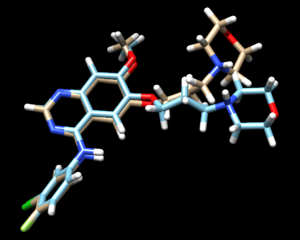
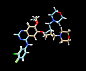
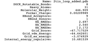
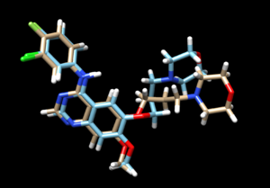
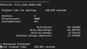
The mol2 file containing the docked ligand could be viewed in ChimeraX under ViewDock. To compare with the reference pose, this mol2 file (blue) has been overlaid on top of the original ligand pose (gold). For this result, it can be seen that although the docking score for the docked ligand is comparable with other docking modes, the RMSD computed for the docked result was larger than 2A, which has been reflected by the pose where the sidechain to the right is shifted further away than in original structure.
The fixed.out file summary the overall docking score of the run:
The steps for the next docking mode should also be similar.
Flexible Docking
In this session, we will be showing the tutorial for Flexible Docking. Among the three docking methods introduced in this tutorial, this would be the most computationally expensive method since the algorithm will be sampling all of the possible conformations of each input ligand and test their binding ability with the binding site. Thus, one might expect the computing time for this method to be exceed other introduced methods.
Please navigate to the directory designated for this docking mode: 008.flex_docking. Here, we can start create the input parameters, file name – flex.in:
vi flex.in
The following is the input parameter for fixed anchor docking. While you can copy and paste this into the body of your script, please make sure to change the input files directory (ligand and protein structure folder) to your personal directory. Also it should be a good practice to make sure the directories for the dock parameters should also be up-to-date.
  conformer_search_type                                        flex
 write_fragment_libraries                                     no
 user_specified_anchor                                        no
 limit_max_anchors                                            no
 min_anchor_size                                              5
 pruning_use_clustering                                       yes
 pruning_max_orients                                          1000
 pruning_clustering_cutoff                                    100
 pruning_conformer_score_cutoff                               100.0
 pruning_conformer_score_scaling_factor                       1.0
 use_clash_overlap                                            no
 write_growth_tree                                            no
 use_internal_energy                                          yes
 internal_energy_rep_exp                                      12
 internal_energy_cutoff                                       100.0
 ligand_atom_file                                             ../004.energy_min/2tio.lig.min_scored.mol2
 limit_max_ligands                                            no
 skip_molecule                                                no
 read_mol_solvation                                           no
 calculate_rmsd                                               yes
 use_rmsd_reference_mol                                       yes
 rmsd_reference_filename                                      ../004.energy_min/2tio.lig.min_scored.mol2
 use_database_filter                                          no
 orient_ligand                                                yes
 automated_matching                                           yes
 receptor_site_file                                           ../002.surface_spheres/selected_spheres.sph
 max_orientations                                             1000
 critical_points                                              no
 chemical_matching                                            no
 use_ligand_spheres                                           no
 bump_filter                                                  no
 score_molecules                                              yes
 contact_score_primary                                        no
 contact_score_secondary                                      no
 grid_score_primary                                           yes
 grid_score_secondary                                         no
 grid_score_rep_rad_scale                                     1
 grid_score_vdw_scale                                         1
 grid_score_es_scale                                          1
 grid_score_grid_prefix                                       ../003.gridbox/grid
 multigrid_score_secondary                                    no
 dock3.5_score_secondary                                      no
 continuous_score_secondary                                   no
 footprint_similarity_score_secondary                         no
 pharmacophore_score_secondary                                no
 descriptor_score_secondary                                   no
 gbsa_zou_score_secondary                                     no
 gbsa_hawkins_score_secondary                                 no
 SASA_score_secondary                                         no
 amber_score_secondary                                        no
 minimize_ligand                                              yes
 minimize_anchor                                              yes
 minimize_flexible_growth                                     yes
 use_advanced_simplex_parameters                              no
 simplex_max_cycles                                           1
 simplex_score_converge                                       0.1
 simplex_cycle_converge                                       1.0
 simplex_trans_step                                           1.0
 simplex_rot_step                                             0.1
 simplex_tors_step                                            10.0
 simplex_anchor_max_iterations                                500
 simplex_grow_max_iterations                                  500
 simplex_grow_tors_premin_iterations                          0
 simplex_random_seed                                          0
 simplex_restraint_min                                        no
 atom_model                                                   all
 vdw_defn_file                                                /gpfs/projects/AMS536/zzz.programs/dock10/parameters/vdw_AMBER_parm99.defn
 flex_defn_file                                               /gpfs/projects/AMS536/zzz.programs/dock10/parameters/flex.defn
 flex_drive_file                                              /gpfs/projects/AMS536/zzz.programs/dock10/parameters/flex_drive.tbl
 ligand_outfile_prefix                                        flex.out
 write_orientations                                           no
 num_scored_conformers                                        1
 rank_ligands                                                 no
Now, you are ready to run dock6 implementing the above input parameters:
dock6 -i flex.in -o flex.out
Dock6 should be running for a couple of minutes. If the program finished right away, it would be recommended that you should check the output file to see if there are any reported errors. Successful run should give you two additional files as followed:
- flex.out
- 2tio_flex.out_scored.mol2
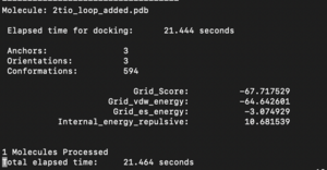
The mol2 file containing the docked ligand could be viewed in ChimeraX under ViewDock. To compare with the reference pose, this mol2 file (blue) has been overlaid on top of the original ligand pose (gold). Under ViewDock in Chimera, it can be observed that the docked ligand showed great structural overlap with the reference pose and this has also been reflected in the reported RMSD score, which has been maintained below 2A.
The fixed.out file summary the overall docking score of the run:
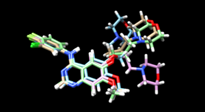
As we have finished running all the docking modes, one step could be carried out here is to compare all the three docked results with the original reference file and see if all the docking results have been suggesting a binding mode that resemble the reference pose. Attached is the overlaid docking results, where we can see the most rigid docking modes give the closest result to the reference structure, whereas fixed anchor docking has the right-side chain shifted further away. Although being the most flexible method, flexible docking gives a good scoring. (gold - original pose, blue - flex, green - rigid, magenta - fixed anchor). Here, you can also open ViewDock, navigate to columns and show grid scores or RMSD score to compare the docking efficiency between the three model, typically, a successful re-dock attempt should have the ligand less than 2A away from the original pose.
Virtual Screening of a Ligand Library
After we have tested our control case for multiple docking modes, in this section we would carry out virtual screening for a larger database of ligands. In this step, the program will attempt to dock all of the input ligands into the binding site and this should be expected to be a time-consuming and computationally exhaustive step. For the purpose of this section, I would be trying out with the 5,000 molecules database, but a safety step you can take is to try running the virtual screening with a smaller subset - containing 100 molecules, to make sure that the program works correctly. The directory to the database of both the 5,000 molecules and 1000 molecules database is available in "gpfs/AMS536/zzz.programs/VS_libraries", there is also a 25,000 molecules subset if you would want to dock to an even larger set. These libraries are extracted from the ZINC library, a commercially available database that contains purchasable chemicals.
Please navigate to the directory designated for virtual screening: 009.virtual_screening. Here, we can start create the input parameters, file name – virutal.in:
vi virtual.in
The following is the input parameter for virtual screening. While you can copy and paste this into the body of your script, please make sure to change the input files directory (ligand and protein structure folder) to your personal directory. Also it should be a good practice to make sure the directories for the dock parameters and the molecule libraries should also be up-to-date.
   conformer_search_type                                        flex
   write_fragment_libraries                                     no
   user_specified_anchor                                        no
   limit_max_anchors                                            no
   min_anchor_size                                              5
   pruning_use_clustering                                       yes
   pruning_max_orients                                          1000
   pruning_clustering_cutoff                                    100
   pruning_conformer_score_cutoff                               100.0
   pruning_conformer_score_scaling_factor                       1.0
   use_clash_overlap                                            no
   write_growth_tree                                            no
   use_internal_energy                                          yes
   internal_energy_rep_exp                                      9
   internal_energy_cutoff                                       100.0
   ligand_atom_file                                             /gpfs/projects/AMS536/zzz.programs/VS_libraries/VS_library_5K.mol2
   limit_max_ligands                                            no
   skip_molecule                                                no
   read_mol_solvation                                           no
   calculate_rmsd                                               no
   use_database_filter                                          no
   orient_ligand                                                yes
   automated_matching                                           yes
   receptor_site_file                                           ../002.surface/selected_spheres.sph
   max_orientations                                             1000
   critical_points                                              no
   chemical_matching                                            no
   use_ligand_spheres                                           no
   bump_filter                                                  no
   score_molecules                                              yes
   contact_score_primary                                        no
   contact_score_secondary                                      no
   grid_score_primary                                           yes
   grid_score_secondary                                         no
   grid_score_rep_rad_scale                                     1
   grid_score_vdw_scale                                         1
   grid_score_es_scale                                          1
   grid_score_grid_prefix                                       ../003.gridbox/grid
   multigrid_score_secondary                                    no
   dock3.5_score_secondary                                      no
   continuous_score_secondary                                   no
   footprint_similarity_score_secondary                         no
   pharmacophore_score_secondary                                no
   descriptor_score_secondary                                   no
   gbsa_zou_score_secondary                                     no
   gbsa_hawkins_score_secondary                                 no
   SASA_score_secondary                                         no
   amber_score_secondary                                        no
   minimize_ligand                                              yes
   minimize_anchor                                              yes
   minimize_flexible_growth                                     yes
   use_advanced_simplex_parameters                              no
   simplex_max_cycles                                           1
   simplex_score_converge                                       0.1
   simplex_cycle_converge                                       1.0
   simplex_trans_step                                           1.0
   simplex_rot_step                                             0.1
   simplex_tors_step                                            10.0
   simplex_anchor_max_iterations                                500
   simplex_grow_max_iterations                                  500
   simplex_grow_tors_premin_iterations                          0
   simplex_random_seed                                          0
   simplex_restraint_min                                        no
   atom_model                                                   all
   vdw_defn_file                                                /gpfs/projects/AMS536/zzz.programs/dock6.10/parameters/vdw_AMBER_parm99.defn
   flex_defn_file                                               /gpfs/projects/AMS536/zzz.programs/dock6.10/parameters/flex.defn
   flex_drive_file                                              /gpfs/projects/AMS536/zzz.programs/dock6.10/parameters/flex_drive.tbl
   ligand_outfile_prefix                                        virtual.out
   write_orientations                                           no
   num_scored_conformers                                        1
   rank_ligands                                                 no
Because the step is time-consuming and might be taking up several hours to run so we will not execute the run on command line but we would submit a job through slurm for this step. In order to do so, we would need to create a job file to submit to the slurm queue:
vi job
The content of the job file should be as followed. In this file, we are running the task on the long-28core that should be compatible with users using login node, if you use other server to submit the task (milan), you should check which core you should be submit to on the SeaWulf website: [1] . We are also using mpirun with 224 partition, you should also change it so that it will fit with the core you are submitting to (if you use a different core).
 #!/bin/bash
 #
 #SBATCH --job-name=2tio_vs_tutorial
 #SBATCH --output=vs_output.txt
 #SBATCH --ntasks-per-node=24
 #SBATCH --nodes=6
 #SBATCH --time=48:00:00
 #SBATCH -p long-28core

 module load intel/mpi/64/2018/18.0.3

 mpirun -np 224 dock6.mpi -i virtual.in -o virtual.out
Close and save the job file and submit the job to slurm with the following command:
sbatch job
You can use the command squeue -u username to check if your job has been submitted, on queue or currently running. The job is expected to take a long while to finish so if the job is executed right away, you should check if there might be a problem in your slurm output file. The output file from this step should be including 3 types of additional files:
- The 2tio.virtual.out_scored.mol2 docked ligand collection.
- The virtual.out file capturing the minimization process - you can check for errors in this file if you cannot run the task. This file is the overall and general output files result from your virtual screening process but you should also see many virtual.out.x files, these files represents each partition from the job that you have indicated on slurm when you are submitting the job.
- The vs_output.txt file.
After you got the result, we can move on to next step of Cartesian minimization and re-scoring steps, and we can view the result at the end.
Cartesian Minimization of Virtually Screened Small Molecules
In this step, we would base on the results we harvested from virtual screening and minimize the energy of the docked structure. Thus, this step would not be as time-consuming as the previous step because it the ligands have already been placed in the binding site of the protein under virtual screening.
Please navigate to the directory designated for Cartesian minimization: 010.cartesian_minimization. Here, we can start create the input parameters, file name – min.in:
vi min.in
The following is the input parameter for virtual screening. While you can copy and paste this into the body of your script, please make sure to change the input files directory (ligand and protein structure folder) to your personal directory.Again here, we want to remind you that you would also be using output from virtual screening so please check if the output of the file is correctly implemented.
 conformer_search_type                                        rigid
 use_internal_energy                                          yes
 internal_energy_rep_exp                                      12
 internal_energy_cutoff                                       100
 ligand_atom_file                                             ../009.virtual_screening/virtual.out_scored.mol2
 limit_max_ligands                                            no
 skip_molecule                                                no
 read_mol_solvation                                           no
 calculate_rmsd                                               no
 use_database_filter                                          no
 orient_ligand                                                no
 bump_filter                                                  no
 score_molecules                                              yes
 contact_score_primary                                        no
 grid_score_primary                                           no
 multigrid_score_primary                                      no
 dock3.5_score_primary                                        no
 continuous_score_primary                                     yes
 cont_score_rec_filename                                      ../001.structure/2tio_protein_hydrogens_charges.mol2
 cont_score_att_exp                                           6
 cont_score_rep_exp                                           12
 cont_score_rep_rad_scale                                     1
 cont_score_use_dist_dep_dielectric                           yes
 cont_score_dielectric                                        4.0
 cont_score_vdw_scale                                         1.0
 cont_score_es_scale                                          1.0
 minimize_ligand                                              yes
 simplex_max_iterations                                       1000
 simplex_tors_premin_iterations                               0
 simplex_max_cycles                                           1.0
 simplex_score_converge                                       0.1
 simplex_cycle_converge                                       1.0
 simplex_trans_step                                           1.0
 simplex_rot_step                                             0.1
 simplex_tors_step                                            10.0
 simplex_random_seed                                          0
 simplex_restraint_min                                        no
 atom_model                                                   all
 vdw_defn_file                                                /gpfs/projects/AMS536/zzz.programs/dock6.10/parameters/vdw_AMBER_parm99.defn
 flex_defn_file                                               /gpfs/projects/AMS536/zzz.programs/dock6.10/parameters/flex.defn
 flex_drive_file                                              /gpfs/projects/AMS536/zzz.programs/dock6.10/parameters/flex_drive.tbl
 ligand_outfile_prefix                                        2tio.virtual_screen.min
 write_orientations                                           no
 num_scored_conformers                                        1
 rank_ligands                                                 no
Although this step is not as exhaustive as the previous step that we have worked on, we would still be submitting the task to slurm because the task is still bulky as we are dealing with 5,000 molecules. In order to do so, we would need to create a job file to submit to the slurm queue:
vi job
The content of the job file should be as followed. As mentioned above, we are running the task on the long-28core that should be compatible with users using login node, if you use other server to submit the task (milan), you should check which core you should be submit to on the SeaWulf website: [2] . We would not be using mpirun to partition like we did with virtual screening because this step is not as bulky.
 #!/bin/bash
 #
 #SBATCH --job-name=2tio_minimization_tutorial
 #SBATCH --output=min_output.txt
 #SBATCH --ntasks-per-node=24
 #SBATCH --nodes=8
 #SBATCH --time=48:00:00
 #SBATCH -p long-28core

 dock6 -i min.in -o min.out
Close and save the job file and submit the job to slurm with the following command:
sbatch job
You can use the command squeue -u username to check if your job has been submitted, on queue or currently running. Similarly if the job finished right away, you should check if there might be a problem in your slurm output file. The output file from this step should be including 3 additional files:
- The 2tio.virtual_screen.min_scored.mol2 docked and minimized ligand collection. - The min.out file capturing the minimization process - you can check for errors in this file if you cannot run the task. - The min_output.txt file.
From here, you can move on the the last step of rescoring the ligand database and viewing your results in Chimera.
Rescoring and Ranking Virtually Screened Molecules
In this step, we would base on the resulting poses of the ligand derived from the previous step where all of the ligands have already been docked and. For this step, not only will we try to re-dock the molecule, but we would also re-rank the molecules based on Footprint Scoring and thus, by comparing these molecules with one another, we would be able to rank which one has the highest potential to be a potential lead.
Please navigate to the directory designated for rescoring the docked ligands: 011.reScore. Here, we can start create the input parameters, file name – rescore.in:
vi rescore.in
The following is the input parameter for virtual screening. While you can copy and paste this into the body of your script, please make sure to change the input files directory (ligand and protein structure folder) to your personal directory. Just like in last step, we would be using output from virtual screening so please check if the output of the file is correctly implemented. Additionally, in order to calculate the footprint similarity score, we would be using the energy minimized structure of the original reference ligand from the 004.energy_min folder, so please make sure the code is pointing to the correct input files.
 conformer_search_type                                         rigid
 use_internal_energy                                          yes
 internal_energy_rep_exp                                      12
 internal_energy_cutoff                                       100
 ligand_atom_file                                             ../009.virtual_screening/virtual.out_scored.mol2
 limit_max_ligands                                            no
 skip_molecule                                                no
 read_mol_solvation                                           no
 calculate_rmsd                                               no
 use_database_filter                                          no
 orient_ligand                                                no
 bump_filter                                                  no
 score_molecules                                              yes
 contact_score_primary                                        no
 contact_score_secondary                                      no
 grid_score_primary                                           no
 grid_score_secondary                                         no
 multigrid_score_primary                                      no
 multigrid_score_secondary                                    no
 dock3.5_score_primary                                        no
 dock3.5_score_secondary                                      no
 continuous_score_primary                                     no
 continuous_score_secondary                                   no
 footprint_similarity_score_primary                           no
 footprint_similarity_score_secondary                         no
 pharmacophore_score_primary                                  no
 pharmacophore_score_secondary                                no
 descriptor_score_primary                                     yes
 descriptor_score_secondary                                   no
 descriptor_use_grid_score                                    no
 descriptor_use_multigrid_score                               no
 descriptor_use_continuous_score                              no
 descriptor_use_footprint_similarity                          yes
 descriptor_use_pharmacophore_score                           yes
 descriptor_use_hungarian                                     yes
 descriptor_use_volume_overlap                                yes
 descriptor_fps_score_use_footprint_reference_mol2            yes
 descriptor_fps_score_footprint_reference_mol2_filename       ../004.energy_min/2tio.lig.min_scored.mol2
 descriptor_fps_score_foot_compare_type                       Euclidean
 descriptor_fps_score_normalize_foot                          no
 descriptor_fps_score_foot_comp_all_residue                   yes
 descriptor_fps_score_receptor_filename                       ../001.structure/2tio_protein_hydrogens_charges.mol2
 descriptor_fps_score_vdw_att_exp                             6
 descriptor_fps_score_vdw_rep_exp                             12
 descriptor_fps_score_vdw_rep_rad_scale                       1
 descriptor_fps_score_use_distance_dependent_dielectric       yes
 descriptor_fps_score_dielectric                              4.0
 descriptor_fps_score_vdw_fp_scale                            1
 descriptor_fps_score_es_fp_scale                             1
 descriptor_fps_score_hb_fp_scale                             0
 descriptor_fms_score_use_ref_mol2                            yes
 descriptor_fms_score_ref_mol2_filename                       ../004.energy_min/2tio.lig.min_scored.mol2
 descriptor_fms_score_write_reference_pharmacophore_mol2      no
 descriptor_fms_score_write_reference_pharmacophore_txt       no
 descriptor_fms_score_write_candidate_pharmacophore           no
 descriptor_fms_score_write_matched_pharmacophore             no
 descriptor_fms_score_compare_type                            overlap
 descriptor_fms_score_full_match                              yes
 descriptor_fms_score_match_rate_weight                       5.0
 descriptor_fms_score_match_dist_cutoff                       1.0
 descriptor_fms_score_match_proj_cutoff                       .7071
 descriptor_fms_score_max_score                               20
 descriptor_fingerprint_ref_filename                          ../004.energy_min/2tio.lig.min_scored.mol2
 descriptor_hms_score_ref_filename                            ../004.energy_min/2tio.lig.min_scored.mol2
 descriptor_hms_score_matching_coeff                          -5
 descriptor_hms_score_rmsd_coeff                              1
 descriptor_volume_score_reference_mol2_filename              ../004.energy_min/2tio.lig.min_scored.mol2
 descriptor_volume_score_overlap_compute_method               analytical
 descriptor_weight_fps_score                                  1
 descriptor_weight_pharmacophore_score                        1
 descriptor_weight_fingerprint_tanimoto                       -1
 descriptor_weight_hms_score                                  1
 descriptor_weight_volume_overlap_score                       -1
 gbsa_zou_score_secondary                                     no
 gbsa_hawkins_score_secondary                                 no
 SASA_score_secondary                                         no
 amber_score_secondary                                        no
 minimize_ligand                                              no
 atom_model                                                   all
 vdw_defn_file                                                /gpfs/projects/AMS536/zzz.programs/dock6.10/parameters/vdw_AMBER_parm99.defn
 flex_defn_file                                               /gpfs/projects/AMS536/zzz.programs/dock6.10/parameters/flex.defn
 flex_drive_file                                              /gpfs/projects/AMS536/zzz.programs/dock6.10/parameters/flex_drive.tbl
 chem_defn_file                                               /gpfs/projects/AMS536/zzz.programs/dock6.10/parameters/chem.defn
 pharmacophore_defn_file                                      /gpfs/projects/AMS536/zzz.programs/dock6.10/parameters/ph4.defn
 ligand_outfile_prefix                                        2tio.output
 write_footprints                                             yes
 write_hbonds                                                 yes
 write_orientations                                           no
 num_scored_conformers                                        1
 rank_ligands                                                 no
For this step, we would also be sending the task to slurm for running. Thus, we would need to create a job file:
vi job
The content of the job file should be as followed. As mentioned above, we are running the task on the long-28core that should be compatible with users using login node, if you use other server to submit the task (milan), you should check which core you should be submit to on the SeaWulf website: [3] . Again, for this step, we would be using 224 partitions with mpirun and you should also re-calculate how many cores would you be using to maximize the runtime efficiency when you put the number down here.
 #!/bin/bash
 #
 #SBATCH --job-name=2tio_rescoring
 #SBATCH --output=rescoring.txt
 #SBATCH --ntasks-per-node=28
 #SBATCH --mail-user=an.p.nguyen@stonybrook.edu
 #SBATCH --nodes=8
 #SBATCH --time=48:00:00
 #SBATCH -p long-28core

 module load intel/mpi/64/2018/18.0.3

 mpirun -np 224 dock6.mpi -i rescore.in -o rescore.out
Close and save the job file and submit the job to slurm with the following command:
sbatch job
You can use the command squeue -u username to check if your job has been submitted, on queue or currently running. Similarly if the job finished right away, you should check if there might be a problem in your slurm output file. The output file from this step should be including 3 additional types of file files:
- The 2tio.output_scored.mol2 docked ligand collection.
- The rescore.out file capturing the rescoring process - you can check for errors in this file if you cannot run the task. This file is the overall and general output files result from your virtual screening process but you should also see many rescore.out.x files, these files represents each partition from the job that you have indicated on slurm so there should in total be 224 rescore.out.x files generated as we have specified that many cores to be using.
- The 2tio.output_footprint_scored.txt, 2tio.output_hbond_scored.txt, and rescoring.txt. The two first .txt files should be showing the scores based on the footprint similarity comparison and the Hydrogen bonds scoring accordingly.
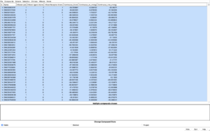
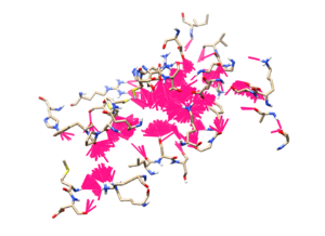
The .mol2 file should be the re-scored and docked structures of the ligands whereas in next step, we would download this file to your local computer and view them in Chimera. To view the results, first, you should open the structure of the protein in Chimera and then open the docked ligands library using ViewDock. Since we are opening a set of 5,000 molecules, the step should take some time to load all the file on to the platform. After the ligands are loaded, in order to view all the ligands on Chimera, you would need to select all the molecules listed on the ViewDock ligands list, you can choose that by selecting the first ligand and scroll down to the bottom of the list and Shift-select the last ligand. Additionally, on the ViewDock window, you can also click on Show > Columns and open as many columns as you want. These columns will then list out the score accordingly, for example, in the attached image, we have shown the number of Hydrogen bonds (combined, ligands', and receptors') and scores (combined score, electrostatic score, and Van der Waals score).
Another viewing process can be done is to go to HBond in ViewDock, and use a bright color to highlight them (in this case we are showing in magenta, with a thicker line option). Next you can go to Action > Inspect and adjust the atom model to show showing the ligand structure itself, along with that set the background to white color and hide the protein's ribbon. The output should be as followed where it would highlight the binding site that the ligands are making contact with.
