Difference between revisions of "2025 DOCK tutorial 1 with PDBID 1O86"
Stonybrook (talk | contribs) (→000: Foundations) |
Stonybrook (talk | contribs) (→007: Footprint Scoring) |
||
| (28 intermediate revisions by the same user not shown) | |||
| Line 21: | Line 21: | ||
===SSH=== | ===SSH=== | ||
You will need to use a Secure Shell (SSH) connection to connect to Seawulf remotely. A guide to this process is [https://rci.stonybrook.edu/HPC/faqs/logging-into-seawulf available on the Seawulf website]. | You will need to use a Secure Shell (SSH) connection to connect to Seawulf remotely. A guide to this process is [https://rci.stonybrook.edu/HPC/faqs/logging-into-seawulf available on the Seawulf website]. | ||
| + | |||
| + | ===Basic Unix Commands and Environment=== | ||
| + | Seawulf uses a terminal-based Unix operating system. If you have never used a terminal-based OS before, you should familiarize yourself with some [https://info-ee.surrey.ac.uk/Teaching/Unix/index.html basic Unix tutorials]. Broadly, you should know how to: | ||
| + | |||
| + | * List your working directory with <code>pwd</code>, change your working directory with <code>cd</code>, make new directories with <code>mkdir</code>, remove directories with <code>rmdir</code>, and list the contents of a directory with <code>ls</code> | ||
| + | * Edit files using the text editor <code>vim</code> (use the <code>vimtutor</code> to read about basic functionality) | ||
| + | * Create an empty file with <code>touch</code>, move files and directories around with <code>mv</code>, copy directories and files with <code>cp</code>, and (very carefully!) remove directories and files with <code>rm</code> | ||
| + | * Determine if commands are available with <code>which</code> | ||
| + | * Understand how to use commands and how flags/input parameters should be formatted | ||
| + | |||
| + | You should also understand the concept of filepaths, and how they are used by commands. Much of DOCK relies on you using the correct filepaths to pass files and parameters into the program, and if the paths are wrong, then the program will not work. When possible, it is advisable to use '''absolute''' filepaths (paths that start at the root directory), as opposed to paths relative to your current working directory. For example, if you are in the directory <code>/gpfs/home/yourusername/tutorial/002_spheres</code>, referencing the absolute path <code>/gpfs/home/yourusername/tutorial/001_structure/important_structure.pdb</code> for a needed structure file is more reliable than the relative path <code>../001_structure/important_structure.pdb</code>, as the latter path is relative to <code>002_spheres/</code>, and meaningless outside of that context. The command <code>realpath</code>will return the absolute path of any file passed to it, which is useful for quickly and accurately determining the absolute path of any file. | ||
| + | |||
| + | To work with DOCK6, it may also be necessary to add a path to your config file that tells Unix where to look for DOCK-related commands. You can check if you need to do this using the command <code>which dock6</code>. If <code>which</code> informs you that no <code>dock6</code> can be found, you will need to edit your .bashrc file: | ||
| + | #Move to your home directory by either entering <code>cd</code> or <code>cd ~</code> | ||
| + | #Use the command <code>vi .bashrc</code> to start editing your personal config file | ||
| + | #At the bottom of the file, add the following line: | ||
| + | <code>export PATH=$PATH:/Path/To/Your/DOCK6/bin</code> | ||
| + | |||
| + | where Path/To/Your/DOCK6/ should be replaced with whatever the path is to your local DOCK installation (note: the full path should end with /bin). At the time of this writing, there is a compiled version of DOCK6.12 at /gpfs/projects/AMS536/zzz.programs/dock6.12_ams536/, but if this does not work then ask Dr. Rizzo or a lab member where a compiled instance can be found | ||
| + | |||
| + | :4. Save and exit the file, then enter the command <code>source .bashrc</code> into the terminal. | ||
| + | :5. Now when you request <code>which dock6</code>, the terminal should return the path to the directory you just provided. | ||
| + | |||
| + | After all this, you should have a good understanding of how to navigate the Unix terminal, and have the DOCK6 suite ready to use in your environment. | ||
| + | |||
| + | === SCP File Transfer === | ||
| + | Another important aspect of working on Seawulf is uploading and downloading files to your local machine. This is accomplished using the Secure Copy Protocol (scp) terminal command. See the pertinent section on the [https://rci.stonybrook.edu/hpc/faqs/transferring-files-to-and-from-seawulf Seawulf website]. For Windows, it may be advisable to download a third party program; [https://filezilla-project.org/ FileZilla] works for this task. | ||
| + | |||
| + | ===Directory setup=== | ||
| + | Finally, assuming all necessary base Unix knowledge has been obtained, you will want to set up a set of directories for the work you will be doing in this tutorial. The directories will help you compartmentalize your work and help to prevent important files from being overwritten or lost. For the modules of this tutorial, we recommend setting up this directory structure, and setting up folders on your local machine with the same names for ease of file transfer: | ||
| + | <code> | ||
| + | ~/001_structure<br> | ||
| + | ~/002_spheres<br> | ||
| + | ~/003_gridbox<br> | ||
| + | ~/004_energy_min<br> | ||
| + | ~/005_rigid_dock<br> | ||
| + | ~/006_flex_dock<br> | ||
| + | ~/007_footprint<br> | ||
| + | ~/008_virtual_screen<br> | ||
| + | ~/009_gen_alg<br> | ||
| + | ~/010_de_novo<br> | ||
| + | </code> | ||
| + | |||
| + | ===A Note on Troubleshooting=== | ||
| + | |||
| + | Finally, despite our best efforts at accuracy, a healthy amount of this tutorial will likely not go smoothly for you. There will be errors and inconsistencies between what you see here and what happens on Seawulf, and there may not be an immediate answer for what you should do to fix them. The instinct when this happens is to find someone who knows what might have happened and ask them for advice, and while this will usually be helpful, it may be inefficient. As such, we advise you to first please ''troubleshoot''. No program you will use in this tutorial is intended to be a black box. All of them do their best to return errors that tell you what is going wrong, and where to look to fix it. If you get an error, read it! Often it will tell you that it can't find a particular file ("doesn't exist" is the favorite wording), or that some piece of the input is giving it trouble— these tell you what paths to check or lines of a file to review. Also, copy-pasting an entire error into Google (or ChatGPT if you must) is a completely valid line of inquiry, and often yields helpful results. | ||
| + | |||
| + | Having said that, here are some common errors and tactics you can use to fix them: | ||
| + | |||
| + | <code>"[File] could not be opened"</code> or <code>"[file] does not exist"</code> usually indicates that a path you gave the program is not accurate. You can "sanity check" paths by copying them directly from the input and putting them into an ls command. If it throws an error, fix the path! | ||
| + | |||
| + | <code>"version `GLIBCXX_whatever' not found"</code> is generally an issue with how the DOCK installation was compiled. Try to find a different version (/gpfs/projects/AMS536/zzz.programs usually has several versions available) or try running the command on a different node (Milan or Login) | ||
| + | |||
| + | Errors mentioning FORTRAAN: Make sure the input files are named correctly(ex INSPH for sphgen) and there are no extra spaces or lines anywhere in the input files. Sometimes they sneak in at the start or end of a line and are parsed literally. | ||
| + | |||
| + | Often, output is sent into a .out file instead of written to the console. If the program terminates immediately but does not return expected files, check whatever .out file was written for errors at the very bottom. | ||
== 001: Structure Prep == | == 001: Structure Prep == | ||
| Line 96: | Line 152: | ||
Explanation of .in for FPS, use of Python script to generate graph | Explanation of .in for FPS, use of Python script to generate graph | ||
| − | == 008: | + | == 008: 5K Virtual Screening == |
| − | Slurm and queue | + | |
| + | In this section, you will conduct a virtual screening on a set of druglike potential leads against the 1O86 receptor. Virtual screening of large ligand libraries is one of the main uses of DOCK and other molecular docking suites in drug discovery, as it allows for lead compound identification at much lower cost than traditional ''in vitro'' assays. | ||
| + | |||
| + | === Input File === | ||
| + | |||
| + | Because this section generates a high volume of molecule poses, you may need to make use of your scratch directory on Seawulf. While your home directory has a maximum storage volume of 20 gigabytes, scratch has a storage volume of 20 TERAbytes, so it will easily accommodate the output of your virtual screen. Your scratch directory should be located at <code>/gpfs/scratch/yourusername/</code>. Move there and create a directory for your virtual screening. | ||
| + | |||
| + | Copy the input file from your <code>006_flex_dock</code> directory into your present directory. We can re-use the majority of input from this file because the docking process is the same in both cases; the only difference is in the number of molecules to be docked. If you like, you can re-name the input file using <code>mv</code> to something like <code>flex_vs.in</code> for clarity. | ||
| + | |||
| + | The only parameter that needs to be changed in the input file is the <code>ligand_atom_file</code> parameter. Instead of the single 1O86 ligand .mol2, we want to dock a .mol2 file that contains multiple potential drug candidates. You should be able to find several such .mol2 files in <code>/gpfs/projects/AMS536/zzz.programs/VS_libraries/</code>. For this tutorial, we will screen the 5,000 molecule library (<code>VS_library_5K.mol2</code>), but you can elect to do the 100- (or 25,000) molecule library by simply changing the input file name. Just copy the path to the file (should be <code>/gpfs/projects/AMS536/zzz.programs/VS_libraries/VS_library_5K.mol2</code>), open the .in file, delete the current value for <code>ligand_atom_file</code>, and paste in the path. If you don't want to deal with the long filepath, you can also copy the VS_library file to your working directory, and just have the filename as the parameter instead. It is probably also advisable to change the names of other output files in the .in file so that the output is distinguishable from the previous flexible docking. | ||
| + | |||
| + | === Slurm and Job Submission === | ||
| + | |||
| + | Up until this point, you have probably been running dock6 on the head node of Seawulf. This is fine for short, low-intensity jobs, like docking a single molecule or (debatably) generating a grid. However, the head node caters to all users currently accessing Seawulf, and has limited computing power at its disposal. As such, attempting to run a longer job (such as a 5,000 molecule screen) will fully consume the head node's limited resources, slowing down or completely killing all user sessions in the process. To safely utilize the full computing power of Seawulf, you need to submit a job to one of its high-powered nodes using its queueing system. This system tracks all jobs that have been submitted by various users and allocates them to processors as they are freed up, maximizing the productivity and efficiency of the computing cluster. The system Seawulf uses for this queue tracking is called Slurm (Simple Linux Utility and Resource Management). | ||
| + | |||
| + | Slurm is implemented as a ''module'' on Seawulf, and needs to be loaded into your environment before it can be used. You can load it by typing <code>module load slurm</code> into your terminal from any directory. Of note, you will need to do this every time you start a new SSH session. If you want the module to always be loaded when you log in, you can add the command to your .bashrc file (see section 000 for instructions on how to modify your .bashrc). | ||
| + | |||
| + | Once the module has loaded, you can use the command <code>sinfo</code> to view what processors are present on Seawulf. If you are on Milan, you should see 40- and 96-core queues of varying lengths (short, medium, long), as well as some specialized GPU cores and high memory cores. The [https://rci.stonybrook.edu/HPC/faqs/seawulf-queues Seawulf website] has some good descriptions of what cores are available and the duration of jobs allowed on them. Adding the <code>--state=idle</code> flag to <code>sinfo</code> allows you to see what queues have cores idle; this is helpful for knowing where a job can start running immediately. | ||
| + | |||
| + | To submit a job to a queue, you need to create a special job script file that will tell the queue everything it needs to know about the job, as well as what commands to run. Here is what one of those files would look like for our VS run: | ||
| + | |||
| + | <nowiki> | ||
| + | #!/bin/bash | ||
| + | # | ||
| + | #SBATCH --job-name=1o86_vs | ||
| + | #SBATCH --output=vs_output.txt | ||
| + | #SBATCH --nodes=1 | ||
| + | #SBATCH --ntasks-per-node=96 | ||
| + | #SBATCH --time=48:00:00 | ||
| + | #SBATCH -p long-96core | ||
| + | |||
| + | module load intel/mpi/64/2018/18.0.3 | ||
| + | |||
| + | dock6.mpi -i flex_vs.in -o flex_vs.out | ||
| + | </nowiki> | ||
| + | |||
| + | A line-by-line breakdown of this file: | ||
| + | * <code>#!/bin/bash</code> is called a shebang, and is used in unix shell scripts to indicate that bash should be used to interpret the script. | ||
| + | * <code>#SBATCH --job-name=1o86_vs</code> tells slurm what our job is called; this can be changed to whatever strikes your fancy without consequence | ||
| + | * <code>#SBATCH --output=vs_output.txt</code> tells slurm where to output information about the job itself. If jobs are not running properly, check this file for errors. | ||
| + | * <code>#SBATCH --nodes=1</code> tells slurm how many computing nodes we want for this job. 1 is appropriate here because we are not using any parallel processing functionality. | ||
| + | * <code>#SBATCH --ntasks-per-node=96</code> tells slurm how many tasks it should expect to run per node. There are no strict guidelines on this, but setting it equal to the number of cores in the node (96 or 40 on Milan) is a good default. | ||
| + | * <code>#SBATCH --time=48:00:00</code> tells slurm the maximum amount of time it should allocate for this job. The best thing to do here is request the maximum time possible for the queue; check the [https://rci.stonybrook.edu/HPC/faqs/seawulf-queues Seawulf website] for each queue's parameters. | ||
| + | * <code>#SBATCH -p long-96core</code> tells slurm which queue we would like to submit to; in this case, we are submitting to the long-term 96-core queue. | ||
| + | * <code>dock6 -i flex_vs.in -o flex_vs.out</code> is the actual command we would like to run in the job. This can be multiple lines of commands, just like a regular shell script, but in this case we are just performing a single virtual screening, so we only call <code>dock6</code> once. | ||
| + | |||
| + | Now that you have a sense of what we're trying to do, create a text file with a recognizable name (ex, job.sh) and either copy-paste or re-type the above input into the file, making any modifications to the dock path or input filename as needed. Save and exit the file. | ||
| + | |||
| + | Finally, you are ready to submit your first job to the queue. Use the command <code>sbatch job.sh</code> to submit your job file. If slurm accepts it, you will be provided a job number. You can use the command <code>squeue -u yourusername</code> to check the status of your job. If you do not see it in the queue directly after submitting, it has likely encountered an error, and you will need to troubleshoot. Otherwise, it will likely start as PD (pending) for a short time before switching to R (running). As it runs, you should see .mol2 files spontaneously created in the directory. Make sure to check semi-regularly that the job is still running. It will likely take 40 hours to finish; if you want to try to speed the process up, you can look at previous tutorials that make use of Message-Passing Interface (MPI) parallelization to use more nodes at once for greater efficiency. | ||
| + | |||
| + | Once the virtual screen has finished, you should have a .mol2 file in your directory that contains the best poses of the 5,000 ligands that were screened, according to purely grid-based docking. | ||
| + | |||
| + | === Re-scoring Docked Molecules === | ||
| + | |||
| + | Although grid scoring provides a good initial look at the most favorable poses of the given molecules, it is generally a good idea to re-score the poses provided by a different criteria to determine a final order. In this case, we will use footprint similarity scoring as our re-scoring function. Once again, we can copy the input file that we used in the single-molecule footprint scoring example, and change the <code>ligand_atom_file</code> parameter from the 1O86 ligand to the output poses from the virtual screening. You should also change <code>ranked_ligands</code> to <code>yes</code> (towards the end of the file), and add a line with the parameter <code>max_ranked_ligands</code> set to <code>500>/code> at the end of the file. This will ensure that the final .mol2 is a manageable size, while retaining the best poses of the docking. Finally, set the <code>ligand_outfile_prefix</code> parameter to something that will distinguish it from the other output already in the directory. Write and exit the file, and rename it to something appropriate like <code>rescore.in</code>. | ||
| + | |||
| + | Because this re-scoring uses rigid docking and no grid calculations, it should be relatively lightweight and safe to run on the head node. If you want to be safe, you can use the command <code>srun -p short-96core -t 1:00:00 –pty bash</code> to instead open up an interactive bash session on one of the computing nodes; this will let you use a terminal live in a manner identical to the head node, but direct all processing requests to an available computing node. Of course, if all the nodes are busy, you will not be able to open an interactive shell on them, so it will be a matter of balancing your patience with your desire for efficiency. | ||
| + | |||
| + | Once you run the re-scoring using <code> dock6 -i rescore.in -o rescore.out</code>, you should see a re-scored ligand file in the directory with the prefix indicated in the rescore.in file. If you want, you can copy this .mol2 file to your home directory so that it is not purged after 30 days (a convenient feature of the scratch directory). After that, download it to your local machine using <code>scp</code>. | ||
| + | |||
| + | |||
| + | === Viewing VS Results in Chimera === | ||
| + | |||
| + | Thanks to our infallible foresight, we have saved only the 500 best ligands to visualize in Chimera, as opposed to the original, crash-inducing number of 5,000. To analyze the poses of these ligands, launch Chimera and File >> Open your receptor .mol2 file. Then, navigate to Tools >> Surface/Binding Analysis >> ViewDock, and open the 500-ligand .mol2 file that you have just downloaded. Chimera may lag for a minute depending on your system specs, but should eventually provide a dialogue box and display one ligand in (hopefully) your receptor's binding site (you can confirm this by re-opening the selected spheres file generated earlier in the tutorial). The dialogue box allows you to select one or multiple ligands at a time to view, and displays their scores in a nice table format. You can view additional columns of data in the dialogue box by navigating to Column >> Show and selecting the desired parameter, and view multiple ligands at a time by clicking one, then holding shift and clicking another. | ||
| + | |||
| + | Congratulations! You have successfully conducted a virtual screening, and now have results for potential lead compounds targeting this receptor. | ||
== 009: Genetic Algorithm Example == | == 009: Genetic Algorithm Example == | ||
| Line 103: | Line 224: | ||
== 010: De Novo Design Example == | == 010: De Novo Design Example == | ||
| − | |||
| + | === De Novo Design === | ||
'''De Novo Design''' is a dock based algorithm that generates new ligands from scratch. This is | '''De Novo Design''' is a dock based algorithm that generates new ligands from scratch. This is | ||
done by selecting a dummy atom, which is the 'seed' that 'grows' scaffolds, linkers, or side chains | done by selecting a dummy atom, which is the 'seed' that 'grows' scaffolds, linkers, or side chains | ||
| Line 114: | Line 235: | ||
will certainly aid in enhancing your search space in generating numerous new compounds. | will certainly aid in enhancing your search space in generating numerous new compounds. | ||
| + | In this tutorial, you will be guided through a '''Denovo refinement calculation'''. This kind of | ||
| + | calculation involves deleting a part of a ligand, creating a dummy atom, and using the De Novo design | ||
| + | algorithm to 'regrow' that part of the ligand based on user defined parameters. | ||
| + | The way in which the 'regrow' process happens comes from the algorithm pulling molecules from fragment libraries | ||
| + | that contain scaffolds, linkers, and sidechains. The user defined parameters will dictate which libraries the | ||
| + | algorithm can pull from. | ||
| + | |||
| + | The outcome will be a series of refinements that will retain a desired interaction in 1O86. | ||
| + | |||
=== Selecting a Dummy Atom === | === Selecting a Dummy Atom === | ||
| Line 160: | Line 290: | ||
First in the terminal, type the command | First in the terminal, type the command | ||
| − | + | vi 1O86_ligand_Du.mol2 | |
Find the C9 atom and modify the atom type. Your input file should look like this: | Find the C9 atom and modify the atom type. Your input file should look like this: | ||
| Line 178: | Line 308: | ||
As a last step, transfer the mol2 to your working directory on seawulf | As a last step, transfer the mol2 to your working directory on seawulf | ||
| − | + | scp 1O86_ligand_Du.mol2 username@login.seawulf.stonybrook.edu:'/gpfs/username/010_de_novo' | |
=== Running The Denovo Calculation === | === Running The Denovo Calculation === | ||
| Line 184: | Line 314: | ||
In your 010_De_Novo folder create an empty input file: | In your 010_De_Novo folder create an empty input file: | ||
| − | + | touch DN.in | |
Then prompt the question tree with the dock program: | Then prompt the question tree with the dock program: | ||
| − | + | dock6 -i DN.in | |
Follow the question tree and use the following sample input file as a template | Follow the question tree and use the following sample input file as a template | ||
| + | |||
| + | conformer_search_type denovo | ||
| + | dn_fraglib_scaffold_file /gpfs/projects/AMS536/zzz.programs/dock6.12_ams536/parameters/fraglib_scaffold.mol2 | ||
| + | dn_fraglib_linker_file /gpfs/projects/AMS536/zzz.programs/dock6.12_ams536/parameters/fraglib_linker.mol2 | ||
| + | dn_fraglib_sidechain_file /gpfs/projects/AMS536/zzz.programs/dock6.12_ams536/parameters/fraglib_sidechain.mol2 | ||
| + | dn_user_specified_anchor yes | ||
| + | dn_fraglib_anchor_file 1O86_ligand_Du.mol2 | ||
| + | dn_torenv_table ../ga_calc/unique_full_sorted_fraglib.dat | ||
| + | dn_name_identifier denovo | ||
| + | dn_sampling_method graph | ||
| + | dn_graph_max_picks 30 | ||
| + | dn_graph_breadth 3 | ||
| + | dn_graph_depth 2 | ||
| + | dn_graph_temperature 100.0 | ||
| + | dn_pruning_conformer_score_cutoff 100.0 | ||
| + | dn_pruning_conformer_score_scaling_factor 2.0 | ||
| + | dn_pruning_clustering_cutoff 100.0 | ||
| + | dn_remove_duplicates yes | ||
| + | dn_max_duplicates_per_mol 0 | ||
| + | dn_write_pruned_duplicates no | ||
| + | dn_advanced_pruning yes | ||
| + | dn_prune_initial_sample yes | ||
| + | dn_sample_torsions yes | ||
| + | dn_prune_individual_torsions yes | ||
| + | dn_prune_combined_torsions yes | ||
| + | dn_random_root_selection no | ||
| + | dn_mol_wt_cutoff_type soft | ||
| + | dn_upper_constraint_mol_wt 1000 | ||
| + | dn_lower_constraint_mol_wt 0.0 | ||
| + | dn_mol_wt_std_dev 35.0 | ||
| + | dn_constraint_rot_bon 15 | ||
| + | dn_constraint_formal_charge 2.0 | ||
| + | dn_heur_unmatched_num 1 | ||
| + | dn_heur_matched_rmsd 2.0 | ||
| + | dn_unique_anchors 1 | ||
| + | dn_max_grow_layers 1 | ||
| + | dn_max_root_size 25 | ||
| + | dn_max_layer_size 25 | ||
| + | dn_max_current_aps 5 | ||
| + | dn_max_scaffolds_per_layer 1 | ||
| + | dn_max_successful_att_per_root 50000 | ||
| + | dn_write_checkpoints yes | ||
| + | dn_write_prune_dump yes | ||
| + | dn_write_orients no | ||
| + | dn_write_growth_trees no | ||
| + | dn_output_prefix DN.out | ||
| + | use_internal_energy yes | ||
| + | internal_energy_rep_exp 12 | ||
| + | internal_energy_cutoff 100.0 | ||
| + | use_database_filter no | ||
| + | orient_ligand no | ||
| + | bump_filter no | ||
| + | score_molecules yes | ||
| + | contact_score_primary no | ||
| + | grid_score_primary yes | ||
| + | grid_score_rep_rad_scale 1 | ||
| + | grid_score_vdw_scale 1 | ||
| + | grid_score_es_scale 1 | ||
| + | grid_lig_efficiency no | ||
| + | grid_score_grid_prefix ../003_gridbox/grid | ||
| + | minimize_ligand yes | ||
| + | minimize_anchor yes | ||
| + | minimize_flexible_growth yes | ||
| + | use_advanced_simplex_parameters no | ||
| + | simplex_max_cycles 1 | ||
| + | simplex_score_converge 0.1 | ||
| + | simplex_cycle_converge 1.0 | ||
| + | simplex_trans_step 1.0 | ||
| + | simplex_rot_step 0.1 | ||
| + | simplex_tors_step 10.0 | ||
| + | simplex_anchor_max_iterations 500 | ||
| + | simplex_grow_max_iterations 500 | ||
| + | simplex_grow_tors_premin_iterations 0 | ||
| + | simplex_final_min no | ||
| + | simplex_random_seed 0 | ||
| + | simplex_restraint_min no | ||
| + | atom_model all | ||
| + | vdw_defn_file /gpfs/projects/AMS536/zzz.programs/dock6.12_ams536/parameters/vdw_AMBER_parm99.defn | ||
| + | flex_defn_file /gpfs/projects/AMS536/zzz.programs/dock6.12_ams536/parameters/flex.defn | ||
| + | flex_drive_file /gpfs/projects/AMS536/zzz.programs/dock6.12_ams536/parameters/flex_drive.tbl | ||
| + | |||
| + | |||
| + | Once you've filled out the input file, you can then go ahead and run the calculation | ||
| + | |||
| + | dock6 -i DN.in -o DN.out | ||
| + | |||
| + | After running the calculations, the following output files will be generated: | ||
| + | |||
| + | DN.out | ||
| + | DN.out.anchor_1.root_layer_1.mol | ||
| + | DN.out.completed.denovo_build.mol2 | ||
| + | DN.out.denovo_build.mol2 | ||
| + | |||
| + | Examining the output file you can see how many molecules were grown. | ||
| + | |||
| + | [[File:Attach_out.png]] | ||
| + | |||
| + | In this case there are 21 different attached molecules. | ||
| + | |||
| + | Now, copy over the DN.out.completed.denovo_build.mol2 to your home computer | ||
| + | |||
| + | scp username@login.seawulf.stonybrook.edu:'/gpfs/username/010_de_novo/DN.out.completed.denovo_build.mol2' . | ||
| + | |||
| + | === Visualizing the Molecules on Chimera === | ||
| + | |||
| + | Head over to Chimera and go to Tools --> Surface/Binding Analysis --> Scroll down to where you see ViewDock and select it | ||
| + | |||
| + | Then select the DN.out.completed_denovo.mol2 | ||
| + | |||
| + | The following menu will appear: | ||
| + | |||
| + | [[File:View_Dock.png]] | ||
| + | |||
| + | You can navigate through the list of molecules that were grown from the calculations. | ||
| + | |||
| + | You'll notice that the best scoring ligand retained the oxygens from the original ligand: | ||
| + | |||
| + | [[File:Best_Scoring_Ligand.png]] | ||
| + | |||
| + | Opening the original ligand mol2, you'll see that the molecules are almost identical | ||
| + | |||
| + | [[File:Overlap_Ligand.png]] | ||
| + | |||
| + | If you return to the ViewDock menu and highlight all of the ligands. | ||
| + | You will be able to see a depiction of all of the ligands that were grown. | ||
| + | |||
| + | This can be done by going to Tools --> ViewDock --> Raise | ||
| + | Now that the menu has been prompted hold down your shift key and select the first ligand, | ||
| + | then scroll down and select the last ligand. All your molecules will be shown overlapping on Chimera: | ||
| + | |||
| + | [[File:Refinements.png]] | ||
| + | |||
| + | Well done, you've now completed a simple denovo calculation! | ||
Revision as of 00:02, 22 February 2025
Contents
DOCK Tutorial using PDB 1O86
[intro text]
000: Foundations
Chimera
UCSF Chimera is a python-based, open-source molecular visualization and manipulation software suite. It is extremely helpful for both preparing molecules/receptors for docking and for visually analyzing the results of those calculations.
It can be downloaded from the official UCSF site; make sure to select the version that matches your operating system (Mac or Windows). Although Chimera is no longer under active development, it remains a relevant software for molecular modeling.
Once Chimera has installed, you can open it to find a blank blue-ish window, with a row of tabs along the top. Throughout this tutorial, you will be instructed to perform different actions contained within these tabs. We will denote the specific tab and sub-tab to be accessed by >> signs. For example, File >> Open PDB would indicate that you should click on the File tab, then mouse to and click Open PDB. This is necessary because some actions are nested in multiple sub-tabs (for instance, selecting all hydrogens in a model would require Select >> Chemistry >> element >> H, as shown below) More extensive documentation on Chimera and its functions is available on the official site.
Seawulf
To complete this tutorial as a Stony Brook student, you will need an account on Seawulf. A ticket to obtain an account can be submitted on the Seawulf website; Dr. Rizzo will need to provide approval for account activation.
The Seawulf website also has a list of best practices for using a High Performance Computing (HPC) cluster. We recommend reading through them before attempting to run any intensive programs on Seawulf.
SSH
You will need to use a Secure Shell (SSH) connection to connect to Seawulf remotely. A guide to this process is available on the Seawulf website.
Basic Unix Commands and Environment
Seawulf uses a terminal-based Unix operating system. If you have never used a terminal-based OS before, you should familiarize yourself with some basic Unix tutorials. Broadly, you should know how to:
- List your working directory with
pwd, change your working directory withcd, make new directories withmkdir, remove directories withrmdir, and list the contents of a directory withls - Edit files using the text editor
vim(use thevimtutorto read about basic functionality) - Create an empty file with
touch, move files and directories around withmv, copy directories and files withcp, and (very carefully!) remove directories and files withrm - Determine if commands are available with
which - Understand how to use commands and how flags/input parameters should be formatted
You should also understand the concept of filepaths, and how they are used by commands. Much of DOCK relies on you using the correct filepaths to pass files and parameters into the program, and if the paths are wrong, then the program will not work. When possible, it is advisable to use absolute filepaths (paths that start at the root directory), as opposed to paths relative to your current working directory. For example, if you are in the directory /gpfs/home/yourusername/tutorial/002_spheres, referencing the absolute path /gpfs/home/yourusername/tutorial/001_structure/important_structure.pdb for a needed structure file is more reliable than the relative path ../001_structure/important_structure.pdb, as the latter path is relative to 002_spheres/, and meaningless outside of that context. The command realpathwill return the absolute path of any file passed to it, which is useful for quickly and accurately determining the absolute path of any file.
To work with DOCK6, it may also be necessary to add a path to your config file that tells Unix where to look for DOCK-related commands. You can check if you need to do this using the command which dock6. If which informs you that no dock6 can be found, you will need to edit your .bashrc file:
- Move to your home directory by either entering
cdorcd ~ - Use the command
vi .bashrcto start editing your personal config file - At the bottom of the file, add the following line:
export PATH=$PATH:/Path/To/Your/DOCK6/bin
where Path/To/Your/DOCK6/ should be replaced with whatever the path is to your local DOCK installation (note: the full path should end with /bin). At the time of this writing, there is a compiled version of DOCK6.12 at /gpfs/projects/AMS536/zzz.programs/dock6.12_ams536/, but if this does not work then ask Dr. Rizzo or a lab member where a compiled instance can be found
- 4. Save and exit the file, then enter the command
source .bashrcinto the terminal. - 5. Now when you request
which dock6, the terminal should return the path to the directory you just provided.
After all this, you should have a good understanding of how to navigate the Unix terminal, and have the DOCK6 suite ready to use in your environment.
SCP File Transfer
Another important aspect of working on Seawulf is uploading and downloading files to your local machine. This is accomplished using the Secure Copy Protocol (scp) terminal command. See the pertinent section on the Seawulf website. For Windows, it may be advisable to download a third party program; FileZilla works for this task.
Directory setup
Finally, assuming all necessary base Unix knowledge has been obtained, you will want to set up a set of directories for the work you will be doing in this tutorial. The directories will help you compartmentalize your work and help to prevent important files from being overwritten or lost. For the modules of this tutorial, we recommend setting up this directory structure, and setting up folders on your local machine with the same names for ease of file transfer:
~/001_structure

~/002_spheres

~/003_gridbox

~/004_energy_min

~/005_rigid_dock

~/006_flex_dock

~/007_footprint

~/008_virtual_screen

~/009_gen_alg

~/010_de_novo
A Note on Troubleshooting
Finally, despite our best efforts at accuracy, a healthy amount of this tutorial will likely not go smoothly for you. There will be errors and inconsistencies between what you see here and what happens on Seawulf, and there may not be an immediate answer for what you should do to fix them. The instinct when this happens is to find someone who knows what might have happened and ask them for advice, and while this will usually be helpful, it may be inefficient. As such, we advise you to first please troubleshoot. No program you will use in this tutorial is intended to be a black box. All of them do their best to return errors that tell you what is going wrong, and where to look to fix it. If you get an error, read it! Often it will tell you that it can't find a particular file ("doesn't exist" is the favorite wording), or that some piece of the input is giving it trouble— these tell you what paths to check or lines of a file to review. Also, copy-pasting an entire error into Google (or ChatGPT if you must) is a completely valid line of inquiry, and often yields helpful results.
Having said that, here are some common errors and tactics you can use to fix them:
"[File] could not be opened" or "[file] does not exist" usually indicates that a path you gave the program is not accurate. You can "sanity check" paths by copying them directly from the input and putting them into an ls command. If it throws an error, fix the path!
"version `GLIBCXX_whatever' not found" is generally an issue with how the DOCK installation was compiled. Try to find a different version (/gpfs/projects/AMS536/zzz.programs usually has several versions available) or try running the command on a different node (Milan or Login)
Errors mentioning FORTRAAN: Make sure the input files are named correctly(ex INSPH for sphgen) and there are no extra spaces or lines anywhere in the input files. Sometimes they sneak in at the start or end of a line and are parsed literally.
Often, output is sent into a .out file instead of written to the console. If the program terminates immediately but does not return expected files, check whatever .out file was written for errors at the very bottom.
001: Structure Prep
Download PDB, separate lig/rec, model loops, addH/charge
Downloading the PDB
Having setup your necessary environment to work on seawulf, lets navigate to your local computer and begin the protein preparation process:
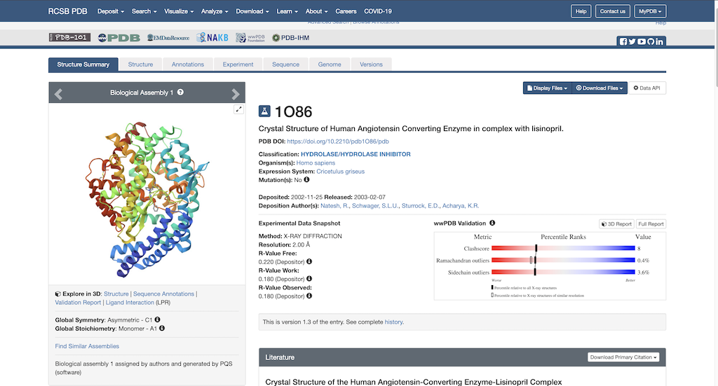
To begin protein preparation you will need the necessary PDB file to work with. Using this link: https://www.rcsb.org/structure/1O86, you will see the RCSB main page opened to our protein of choice:
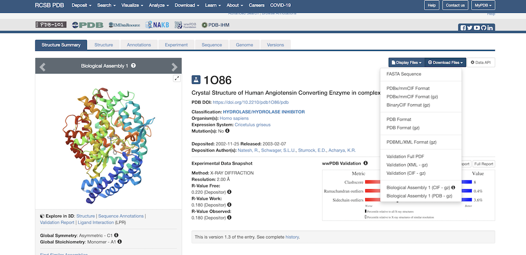
Next, you'll want to navigate to the top right corner where it says Download Files. Then, select the dropdown arrow. The following pulldown menu will appear on the screen:
Select 'Download PDB'. Now the PDB file is downloaded to your local computer.
Now that you have the PDB file, lets navigate to Chimera program to open the file.
002: Spheres
surface generation, sphgen, selecting spheres, visualization in Chimera
Generate the required surface file
1. Open 1O86 protein only file in chimera and hit select > show> surface 2. Write the DMS file by choosing tools>structure editing>Write DMS 3. Upload the DMS file to your directory 4. Create a sphere input file using the following command:
vi INSPH
5. Paste the following into your input file:
./IO86.dms
R
X
0.0
4.0
1.4
IO86.sph
6. Run the program with the following command
sphgen -i INSPH -o OUTSPH
7. Download the output file to your local directory and open and overlay with protein file in Chimera File:Screenshot 2025-02-19 130820.png
Based on the overlay the ribbons are aligned with the spheres indicating the generation of surface spheres was successful.
Generate Spheres localized on binding site
003: Grid/box
showbox, grid generation, visualization in Chimera
004: Minimization
Explanation of .in file for minimization and process (Chimera visuals after)
005: Rigid Docking
Explanation of .in file for rigid docking and process (Chimera visuals after)
006: Flexible Docking
Explanation of .in for flex docking (Chimera visuals after)
007: Footprint Scoring
Explanation of .in for FPS, use of Python script to generate graph
008: 5K Virtual Screening
In this section, you will conduct a virtual screening on a set of druglike potential leads against the 1O86 receptor. Virtual screening of large ligand libraries is one of the main uses of DOCK and other molecular docking suites in drug discovery, as it allows for lead compound identification at much lower cost than traditional in vitro assays.
Input File
Because this section generates a high volume of molecule poses, you may need to make use of your scratch directory on Seawulf. While your home directory has a maximum storage volume of 20 gigabytes, scratch has a storage volume of 20 TERAbytes, so it will easily accommodate the output of your virtual screen. Your scratch directory should be located at /gpfs/scratch/yourusername/. Move there and create a directory for your virtual screening.
Copy the input file from your 006_flex_dock directory into your present directory. We can re-use the majority of input from this file because the docking process is the same in both cases; the only difference is in the number of molecules to be docked. If you like, you can re-name the input file using mv to something like flex_vs.in for clarity.
The only parameter that needs to be changed in the input file is the ligand_atom_file parameter. Instead of the single 1O86 ligand .mol2, we want to dock a .mol2 file that contains multiple potential drug candidates. You should be able to find several such .mol2 files in /gpfs/projects/AMS536/zzz.programs/VS_libraries/. For this tutorial, we will screen the 5,000 molecule library (VS_library_5K.mol2), but you can elect to do the 100- (or 25,000) molecule library by simply changing the input file name. Just copy the path to the file (should be /gpfs/projects/AMS536/zzz.programs/VS_libraries/VS_library_5K.mol2), open the .in file, delete the current value for ligand_atom_file, and paste in the path. If you don't want to deal with the long filepath, you can also copy the VS_library file to your working directory, and just have the filename as the parameter instead. It is probably also advisable to change the names of other output files in the .in file so that the output is distinguishable from the previous flexible docking.
Slurm and Job Submission
Up until this point, you have probably been running dock6 on the head node of Seawulf. This is fine for short, low-intensity jobs, like docking a single molecule or (debatably) generating a grid. However, the head node caters to all users currently accessing Seawulf, and has limited computing power at its disposal. As such, attempting to run a longer job (such as a 5,000 molecule screen) will fully consume the head node's limited resources, slowing down or completely killing all user sessions in the process. To safely utilize the full computing power of Seawulf, you need to submit a job to one of its high-powered nodes using its queueing system. This system tracks all jobs that have been submitted by various users and allocates them to processors as they are freed up, maximizing the productivity and efficiency of the computing cluster. The system Seawulf uses for this queue tracking is called Slurm (Simple Linux Utility and Resource Management).
Slurm is implemented as a module on Seawulf, and needs to be loaded into your environment before it can be used. You can load it by typing module load slurm into your terminal from any directory. Of note, you will need to do this every time you start a new SSH session. If you want the module to always be loaded when you log in, you can add the command to your .bashrc file (see section 000 for instructions on how to modify your .bashrc).
Once the module has loaded, you can use the command sinfo to view what processors are present on Seawulf. If you are on Milan, you should see 40- and 96-core queues of varying lengths (short, medium, long), as well as some specialized GPU cores and high memory cores. The Seawulf website has some good descriptions of what cores are available and the duration of jobs allowed on them. Adding the --state=idle flag to sinfo allows you to see what queues have cores idle; this is helpful for knowing where a job can start running immediately.
To submit a job to a queue, you need to create a special job script file that will tell the queue everything it needs to know about the job, as well as what commands to run. Here is what one of those files would look like for our VS run:
#!/bin/bash
#
#SBATCH --job-name=1o86_vs
#SBATCH --output=vs_output.txt
#SBATCH --nodes=1
#SBATCH --ntasks-per-node=96
#SBATCH --time=48:00:00
#SBATCH -p long-96core

module load intel/mpi/64/2018/18.0.3

dock6.mpi -i flex_vs.in -o flex_vs.out
A line-by-line breakdown of this file:
-
#!/bin/bashis called a shebang, and is used in unix shell scripts to indicate that bash should be used to interpret the script. -
#SBATCH --job-name=1o86_vstells slurm what our job is called; this can be changed to whatever strikes your fancy without consequence -
#SBATCH --output=vs_output.txttells slurm where to output information about the job itself. If jobs are not running properly, check this file for errors. -
#SBATCH --nodes=1tells slurm how many computing nodes we want for this job. 1 is appropriate here because we are not using any parallel processing functionality. -
#SBATCH --ntasks-per-node=96tells slurm how many tasks it should expect to run per node. There are no strict guidelines on this, but setting it equal to the number of cores in the node (96 or 40 on Milan) is a good default. -
#SBATCH --time=48:00:00tells slurm the maximum amount of time it should allocate for this job. The best thing to do here is request the maximum time possible for the queue; check the Seawulf website for each queue's parameters. -
#SBATCH -p long-96coretells slurm which queue we would like to submit to; in this case, we are submitting to the long-term 96-core queue. -
dock6 -i flex_vs.in -o flex_vs.outis the actual command we would like to run in the job. This can be multiple lines of commands, just like a regular shell script, but in this case we are just performing a single virtual screening, so we only calldock6once.
Now that you have a sense of what we're trying to do, create a text file with a recognizable name (ex, job.sh) and either copy-paste or re-type the above input into the file, making any modifications to the dock path or input filename as needed. Save and exit the file.
Finally, you are ready to submit your first job to the queue. Use the command sbatch job.sh to submit your job file. If slurm accepts it, you will be provided a job number. You can use the command squeue -u yourusername to check the status of your job. If you do not see it in the queue directly after submitting, it has likely encountered an error, and you will need to troubleshoot. Otherwise, it will likely start as PD (pending) for a short time before switching to R (running). As it runs, you should see .mol2 files spontaneously created in the directory. Make sure to check semi-regularly that the job is still running. It will likely take 40 hours to finish; if you want to try to speed the process up, you can look at previous tutorials that make use of Message-Passing Interface (MPI) parallelization to use more nodes at once for greater efficiency.
Once the virtual screen has finished, you should have a .mol2 file in your directory that contains the best poses of the 5,000 ligands that were screened, according to purely grid-based docking.
Re-scoring Docked Molecules
Although grid scoring provides a good initial look at the most favorable poses of the given molecules, it is generally a good idea to re-score the poses provided by a different criteria to determine a final order. In this case, we will use footprint similarity scoring as our re-scoring function. Once again, we can copy the input file that we used in the single-molecule footprint scoring example, and change the ligand_atom_file parameter from the 1O86 ligand to the output poses from the virtual screening. You should also change ranked_ligands to yes (towards the end of the file), and add a line with the parameter max_ranked_ligands set to 500>/code> at the end of the file. This will ensure that the final .mol2 is a manageable size, while retaining the best poses of the docking. Finally, set the <code>ligand_outfile_prefix parameter to something that will distinguish it from the other output already in the directory. Write and exit the file, and rename it to something appropriate like rescore.in.
Because this re-scoring uses rigid docking and no grid calculations, it should be relatively lightweight and safe to run on the head node. If you want to be safe, you can use the command srun -p short-96core -t 1:00:00 –pty bash to instead open up an interactive bash session on one of the computing nodes; this will let you use a terminal live in a manner identical to the head node, but direct all processing requests to an available computing node. Of course, if all the nodes are busy, you will not be able to open an interactive shell on them, so it will be a matter of balancing your patience with your desire for efficiency.
Once you run the re-scoring using dock6 -i rescore.in -o rescore.out, you should see a re-scored ligand file in the directory with the prefix indicated in the rescore.in file. If you want, you can copy this .mol2 file to your home directory so that it is not purged after 30 days (a convenient feature of the scratch directory). After that, download it to your local machine using scp.
Viewing VS Results in Chimera
Thanks to our infallible foresight, we have saved only the 500 best ligands to visualize in Chimera, as opposed to the original, crash-inducing number of 5,000. To analyze the poses of these ligands, launch Chimera and File >> Open your receptor .mol2 file. Then, navigate to Tools >> Surface/Binding Analysis >> ViewDock, and open the 500-ligand .mol2 file that you have just downloaded. Chimera may lag for a minute depending on your system specs, but should eventually provide a dialogue box and display one ligand in (hopefully) your receptor's binding site (you can confirm this by re-opening the selected spheres file generated earlier in the tutorial). The dialogue box allows you to select one or multiple ligands at a time to view, and displays their scores in a nice table format. You can view additional columns of data in the dialogue box by navigating to Column >> Show and selecting the desired parameter, and view multiple ligands at a time by clicking one, then holding shift and clicking another.
Congratulations! You have successfully conducted a virtual screening, and now have results for potential lead compounds targeting this receptor.
009: Genetic Algorithm Example
Explanation of rationale for GA and basic functionality, sample input file and expected outputs
010: De Novo Design Example
De Novo Design
De Novo Design is a dock based algorithm that generates new ligands from scratch. This is done by selecting a dummy atom, which is the 'seed' that 'grows' scaffolds, linkers, or side chains based on user defined parameters. For example, say you only wanted to use de novo design to only 'grow' drug-like molecules. The way this is accomplished is ensuring the input file contains parameters that bias the algorithm to abide by Lipinski's Rule of 5 The guiding principle for using De Novo design is because there is a limit to the amount of new molecules that you could generate using a general virtual screening. Nevertheless, this method will certainly aid in enhancing your search space in generating numerous new compounds.
In this tutorial, you will be guided through a Denovo refinement calculation. This kind of calculation involves deleting a part of a ligand, creating a dummy atom, and using the De Novo design algorithm to 'regrow' that part of the ligand based on user defined parameters. The way in which the 'regrow' process happens comes from the algorithm pulling molecules from fragment libraries that contain scaffolds, linkers, and sidechains. The user defined parameters will dictate which libraries the algorithm can pull from.
The outcome will be a series of refinements that will retain a desired interaction in 1O86.
Selecting a Dummy Atom
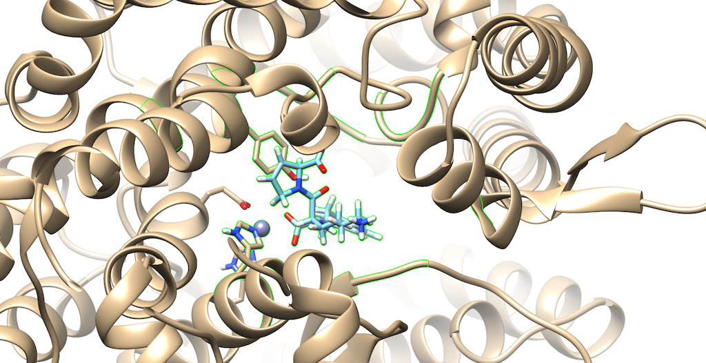
To prepare our molecule for a De Novo calculation, we must first select a dummy atom to 'grow' from. To do this, first open your 1O86_fixed_protein_H_cH.mol2 file, then your 1O86_ligand_H_cH.mol2. The rationale for this is we would like to delete an atom on the ligand that contains a group that interacts with the protein. This will help to produce meaningful results, from a drug design standpoint:
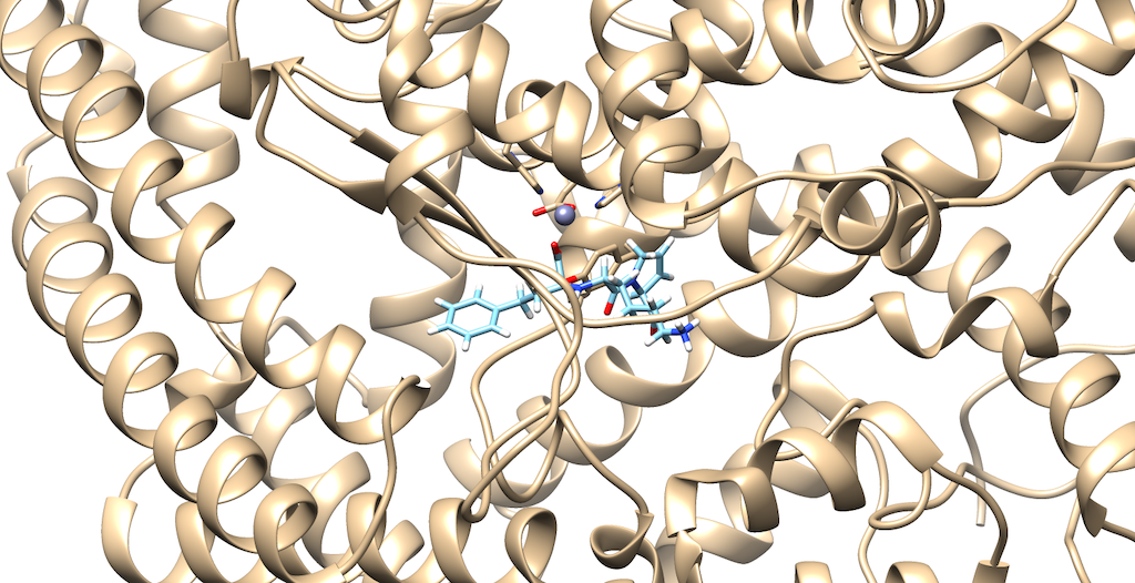
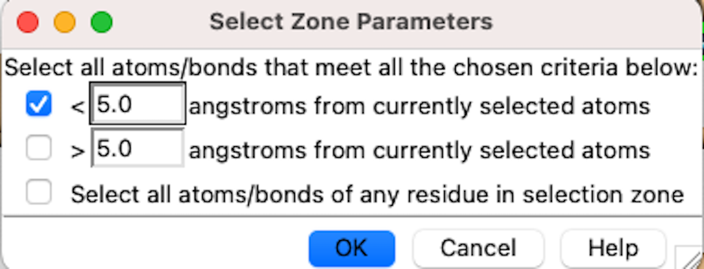
As you can see it is a little difficult to see which atoms are interacting with the protein. To refine this inspection, hit Control and select an atom on the ligand. Then, hit the up arrow to highlight the entire ligand. Next, hit Select --> Zone and the following menu appears:
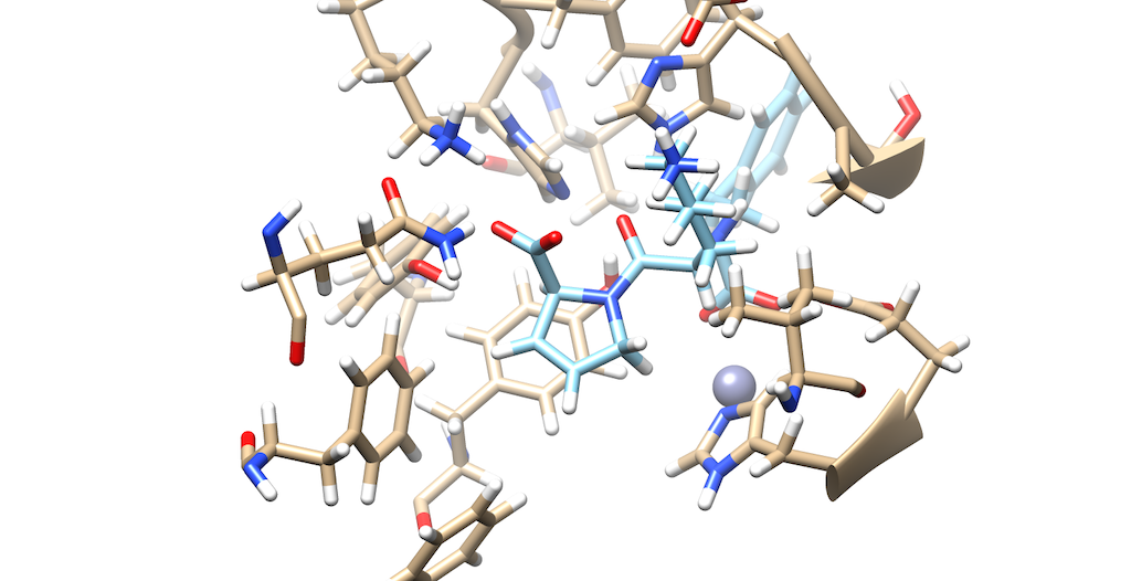
Lets modify the Zone and change the number from 5.0 angstroms to 3.0 angstroms. Additionally, make sure that that the third box is checked off entitled that selects neighboring residues. Then, press okay. You will notice that your ligand and the neighboring residues are highlighted:
To modify this image even further: Go to Actions --> Atoms/Bonds --> hit Show Next, navigate to Select --> press Invert(selected models), here you'll notice most of the protein is highlighted Lastly, Return to Actions --> Atoms/Bonds --> hit delete You now see that there is a clearer picture of specifically, which atoms are interacting closely with the protein
You'll notice that there are two oxygens interacting with neighboring residues in the protein. Tracing your cursor in between the oxygens, you'll highlight a Carbon atom labeled C9. This will be the atom of choice for this tutorial.
Generating a Dummy Atom
Now that we have our atom of choice, we need to modify the ligand as well as the mol2 file itself.
First, open the 1O86_ligand_H_cH.mol2 in Chimera.
Locate the C9 atom --> select the two oxygens attached to C9 --> Atoms/Bonds --> delete. Then, save the mol2 file, lets call it 1O86_ligand_Du.mol2.
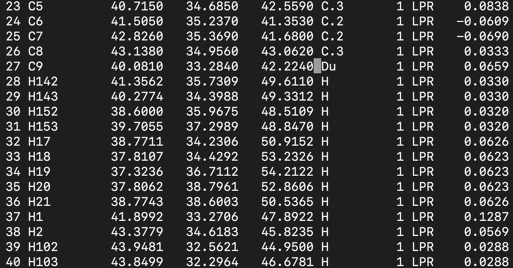
Finally, we must open the mol2 file on our terminal and change the atom type of C9 to Du:
First in the terminal, type the command
vi 1O86_ligand_Du.mol2
Find the C9 atom and modify the atom type. Your input file should look like this:
Save it.
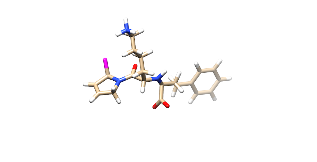
Now lets verify this change by opening the mol2 file on Chimera:
As you can see C9 is now a dummy atom as shown in purple
Now, the mol2 is ready for De Novo calculations
As a last step, transfer the mol2 to your working directory on seawulf
scp 1O86_ligand_Du.mol2 username@login.seawulf.stonybrook.edu:'/gpfs/username/010_de_novo'
Running The Denovo Calculation
In your 010_De_Novo folder create an empty input file:
touch DN.in
Then prompt the question tree with the dock program:
dock6 -i DN.in
Follow the question tree and use the following sample input file as a template
  conformer_search_type                                        denovo
  dn_fraglib_scaffold_file                                     /gpfs/projects/AMS536/zzz.programs/dock6.12_ams536/parameters/fraglib_scaffold.mol2
  dn_fraglib_linker_file                                       /gpfs/projects/AMS536/zzz.programs/dock6.12_ams536/parameters/fraglib_linker.mol2
  dn_fraglib_sidechain_file                                    /gpfs/projects/AMS536/zzz.programs/dock6.12_ams536/parameters/fraglib_sidechain.mol2
  dn_user_specified_anchor                                     yes
  dn_fraglib_anchor_file                                       1O86_ligand_Du.mol2
  dn_torenv_table                                              ../ga_calc/unique_full_sorted_fraglib.dat
  dn_name_identifier                                           denovo
  dn_sampling_method                                           graph
  dn_graph_max_picks                                           30
  dn_graph_breadth                                             3
  dn_graph_depth                                               2
  dn_graph_temperature                                         100.0
  dn_pruning_conformer_score_cutoff                            100.0
  dn_pruning_conformer_score_scaling_factor                    2.0
  dn_pruning_clustering_cutoff                                 100.0
  dn_remove_duplicates                                         yes
  dn_max_duplicates_per_mol                                    0
  dn_write_pruned_duplicates                                   no
  dn_advanced_pruning                                          yes
  dn_prune_initial_sample                                      yes
  dn_sample_torsions                                           yes
  dn_prune_individual_torsions                                 yes
  dn_prune_combined_torsions                                   yes
  dn_random_root_selection                                     no
  dn_mol_wt_cutoff_type                                        soft
  dn_upper_constraint_mol_wt                                   1000
  dn_lower_constraint_mol_wt                                   0.0
  dn_mol_wt_std_dev                                            35.0
  dn_constraint_rot_bon                                        15
  dn_constraint_formal_charge                                  2.0
  dn_heur_unmatched_num                                        1
  dn_heur_matched_rmsd                                         2.0
  dn_unique_anchors                                            1
  dn_max_grow_layers                                           1
  dn_max_root_size                                             25
  dn_max_layer_size                                            25
  dn_max_current_aps                                           5
  dn_max_scaffolds_per_layer                                   1
  dn_max_successful_att_per_root                               50000
  dn_write_checkpoints                                         yes
  dn_write_prune_dump                                          yes
  dn_write_orients                                             no
  dn_write_growth_trees                                        no
  dn_output_prefix                                             DN.out
  use_internal_energy                                          yes
  internal_energy_rep_exp                                      12
  internal_energy_cutoff                                       100.0
  use_database_filter                                          no
  orient_ligand                                                no
  bump_filter                                                  no
  score_molecules                                              yes
  contact_score_primary                                        no
  grid_score_primary                                           yes
  grid_score_rep_rad_scale                                     1
  grid_score_vdw_scale                                         1
  grid_score_es_scale                                          1
  grid_lig_efficiency                                          no
  grid_score_grid_prefix                                       ../003_gridbox/grid
  minimize_ligand                                              yes
  minimize_anchor                                              yes
  minimize_flexible_growth                                     yes
  use_advanced_simplex_parameters                              no
  simplex_max_cycles                                           1
  simplex_score_converge                                       0.1
  simplex_cycle_converge                                       1.0
  simplex_trans_step                                           1.0
  simplex_rot_step                                             0.1
  simplex_tors_step                                            10.0
  simplex_anchor_max_iterations                                500
  simplex_grow_max_iterations                                  500
  simplex_grow_tors_premin_iterations                          0
  simplex_final_min                                            no
  simplex_random_seed                                          0
  simplex_restraint_min                                        no
  atom_model                                                   all
  vdw_defn_file                                                /gpfs/projects/AMS536/zzz.programs/dock6.12_ams536/parameters/vdw_AMBER_parm99.defn
  flex_defn_file                                               /gpfs/projects/AMS536/zzz.programs/dock6.12_ams536/parameters/flex.defn
  flex_drive_file                                              /gpfs/projects/AMS536/zzz.programs/dock6.12_ams536/parameters/flex_drive.tbl
Once you've filled out the input file, you can then go ahead and run the calculation
dock6 -i DN.in -o DN.out
After running the calculations, the following output files will be generated:
 DN.out
 DN.out.anchor_1.root_layer_1.mol
 DN.out.completed.denovo_build.mol2
 DN.out.denovo_build.mol2
Examining the output file you can see how many molecules were grown.
In this case there are 21 different attached molecules.
Now, copy over the DN.out.completed.denovo_build.mol2 to your home computer
scp username@login.seawulf.stonybrook.edu:'/gpfs/username/010_de_novo/DN.out.completed.denovo_build.mol2' .
Visualizing the Molecules on Chimera
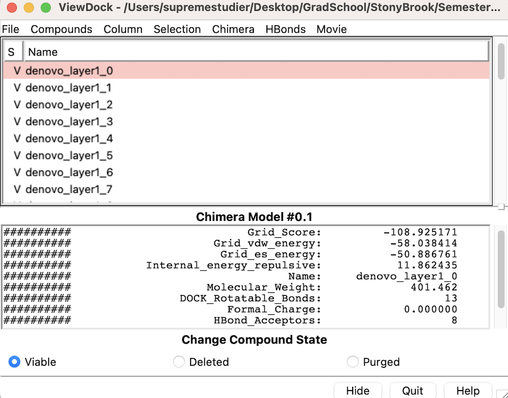
Head over to Chimera and go to Tools --> Surface/Binding Analysis --> Scroll down to where you see ViewDock and select it
Then select the DN.out.completed_denovo.mol2
The following menu will appear:
You can navigate through the list of molecules that were grown from the calculations.
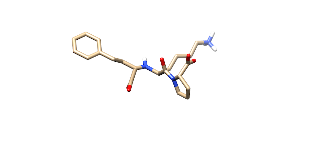
You'll notice that the best scoring ligand retained the oxygens from the original ligand:
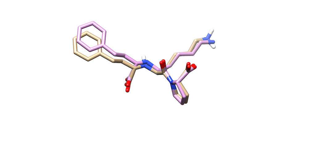
Opening the original ligand mol2, you'll see that the molecules are almost identical
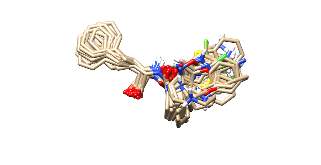
If you return to the ViewDock menu and highlight all of the ligands. You will be able to see a depiction of all of the ligands that were grown.
This can be done by going to Tools --> ViewDock --> Raise Now that the menu has been prompted hold down your shift key and select the first ligand, then scroll down and select the last ligand. All your molecules will be shown overlapping on Chimera:
Well done, you've now completed a simple denovo calculation!
