Difference between revisions of "2023 DOCK tutorial 1 with PDBID 4S0V"
Stonybrook (talk | contribs) (→Downloading a protein from the PDB database) |
(→Virtual Screening of a Ligand Library) |
||
| (244 intermediate revisions by 2 users not shown) | |||
| Line 3: | Line 3: | ||
The following steps will be followed: | The following steps will be followed: | ||
| − | #Setting up your | + | #Setting up your environment |
#Downloading a protein from the PDB database | #Downloading a protein from the PDB database | ||
| − | #Determining if there are any missing loops and if they need to be modeled | + | #Determining if there are any missing loops in the structure and if they need to be modeled |
#Preparing the ligand | #Preparing the ligand | ||
#Preparing the protein | #Preparing the protein | ||
| + | #Finding the binding site of the protein | ||
| + | |||
| + | |||
| + | You will need certain skills to successfully complete this tutorial. This website has tutorials for the following: | ||
| + | *[http://ringo.ams.stonybrook.edu/index.php/Unix UNIX] | ||
| + | *[http://ringo.ams.stonybrook.edu/index.php/Chimera Chimera] | ||
| + | *[http://ringo.ams.stonybrook.edu/index.php/Vi vi] | ||
| + | |||
| + | This tutorial will be using PDB#4S0V as an example. Keep in mind that when you work on your own project to replace any reference to 4S0V with your own protein number. | ||
== Learning Objectives == | == Learning Objectives == | ||
| Line 14: | Line 23: | ||
== Setting Up Your Environment == | == Setting Up Your Environment == | ||
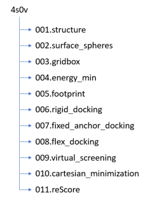
| + | Before we get started working with molecules it's a good idea to set up your directory structure on Seawulf to keep everything organized. The following directory structure should be created: | ||
| + | [[File: 4s0v_directoryStructure.png|thumb|center]] | ||
| + | |||
| + | == Downloading a protein from the PDB database == | ||
| + | The first step is to download a protein complex from the [https://rcsb.org/ PDB]. As mentioned, this tutorial will be using #4S0V throughout. On the right side of the top banner you will see a search bar: | ||
| + | |||
| + | [[File:searchbar.png|center|thumb|upright=2.0]]. | ||
| + | |||
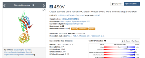
| + | Simply type in 4S0V and press enter. The resulting protein complex will be displayed. | ||
| + | [[File:landing.png|center|500px]] | ||
| − | |||
| − | |||
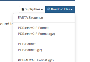
| − | That's it! The pdb file | + | On the right hand side, click on Download Files, then choose PDB Format. |
| + | [[File:downloads.png|center|300px]] | ||
| + | |||
| + | That's it! The pdb file is now saved to your local computer. | ||
= Preparation of the ligand and protein = | = Preparation of the ligand and protein = | ||
| + | The following steps will show you how to prepare the protein and ligand structures to be used with DOCK. All steps in this section will be done using Chimera. These steps are very important - if your initial structure is not prepared properly, all downstream analysis can potentially be incorrect. This section will show you how to: | ||
| + | #Evaluate the structure to determine if there are any missing loops | ||
| + | #Prepare the protein structure | ||
| + | #Prepare the ligand structure | ||
| + | |||
=== Evaluating the Structure=== | === Evaluating the Structure=== | ||
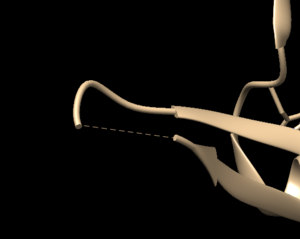
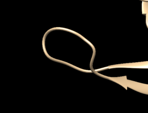
| + | Open the previously downloaded .pdb file into Chimera. The first thing you want to look for are missing loops. A missing loop will be indicated by a dashed line in the structure: | ||
| + | [[File:missingloop.png|thumb|center]] | ||
| + | |||
| + | The first decision you'll need to make is if these missing loops are important in your model. This decision is made by determining if the missing loop is close to the binding site. If it is far enough away, it probably won't affect the dynamics of the protein/ligand interaction and can be left alone. If the missing section is close to the binding site, you may want to fix it to more accurately model the binding site and the protein/ligand interaction. | ||
| + | |||
| + | To determine the distance between the missing loop and the binding site: | ||
| + | #Select an atom at near the start of the missing section (hold the ctrl button while clicking it) | ||
| + | #Select another atom near the binding site (hold ctrl + shift while clicking the second atom) | ||
| + | #Go to Tools → Structure Analysis → Distances | ||
| + | |||
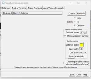
| + | A dialogue box will appear: | ||
| + | [[File: distances.png|thumb|center]] | ||
| + | |||
| + | Click the 'create' button and the distances between the two selected atoms will appear in the box. With this box open you can clear your selection (Select → Clear Selection) and then choose two more atoms. When 'Create' is again pressed, the second distance will be added to the dialogue box. | ||
| + | |||
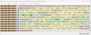
| + | If you determine that you want to re-create the missing sections, go to Tools → Surface Editing → Model/Refine Loops. Two dialogue boxes will appear: | ||
| + | [[File: sequence.png|thumb|center]] | ||
| + | |||
| + | this box shows the sequence of amino acids in your structure. | ||
| + | |||
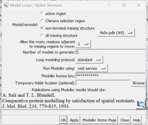
| + | The second box is the important one for this step. This has the required inputs you need to give Chimera so it can re-model the missing loops: | ||
| + | |||
| + | [[File: inputmissing.png|thumb|center]] | ||
| + | |||
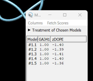
| + | in this box choose 'non-terminal missing structure' and click 'Apply'. You can monitor the progress of Modeller in the lower left hand corner of the display. Once it has finished, another dialogue box will appear showing you the five choices of models for the missing sections. | ||
| + | |||
| + | [[File:loopchoice.png|thumb|center]] | ||
| + | |||
| + | As you click on each of the results, the re-created missing section will show up. Decide which one you want to keep, highlight it and save the file by choosing File → Save PDB. In the dialogue box, be sure to give this file a new name so as not to overwrite the original 4s0v.pdb file, something similar to 4s0v_loops_fixed.pdb. In the 'Save models' section, choose the model number you chose above. To confirm that everything has worked correctly, close your current session in Chimera and open 4s0v_loops_fixed.pdb. You should now see no dashed lines and only the structure with the re-created loops. | ||
| + | [[File:fixed.png|thumb|center]] | ||
| + | You are now ready to move onto preparing the ligand and protein structures for docking. | ||
===Preparing the Protein file=== | ===Preparing the Protein file=== | ||
| + | The first step in preparing the protein is to get the protein structure alone in a .pdb file. To do this: | ||
| + | #Select an atom on the protein | ||
| + | #Press the up arrow until the entire protein is selected | ||
| + | #Go to Select → Invert (all models). This will change the selection from the protein to everything else in the structure | ||
| + | #Go to Actions → Atoms/Bonds → Delete | ||
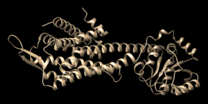
| + | #Save the structure with a new file name (i.e. 4s0v_protein_only.pdb). Your pdb file will now look similar to this: | ||
| + | [[File: proteinonly.png|thumb|center]] | ||
| + | |||
| + | At this point we also need to generate a .mol2 file for the structure in this state. Go to File → Save Mol2 and give the file a descriptive name such as 4s0v_protein_no_hydrogens_no_charges.mol2 | ||
| + | There are now two more steps necessary for its preparation: | ||
| + | #Adding hydrogens | ||
| + | #Adding charge | ||
| + | |||
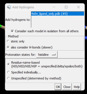
| + | To add hydrogen atoms click on: Tools → Structure Editing → AddH. This command will cause the following dialogue box to appear: | ||
| + | [[File: addhs.png|thumb|center]] | ||
| + | |||
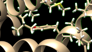
| + | Click 'OK'. When the program is finished, the bottom left-hand side will say "Hydrogens added" but you won't see any change in the structure. It's good practice to make sure that the program worked properly by showing the atoms at a small area of the protein and ensuring hydrogens were added. To do with we're going to use the 'zone' command which is quite useful: | ||
| + | #Click on one atom anywhere on the protein | ||
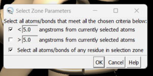
| + | #Click on Select → Zone. This will cause the following dialogue box to appear: | ||
| + | [[File: zoneselection.png|thumb|center]] | ||
| + | |||
| + | make sure to click the same options as shown above and click on 'OK'. Go to Actions → Atoms/Bonds → show and the atoms in the atoms in the selected area will be shown. If the hydrogen atoms were successfully added you'll see structure similar to: | ||
| + | [[File: honprotein.png|thumb|center]] | ||
| + | |||
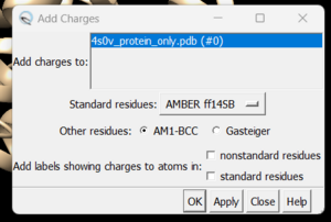
| + | and you can see the white ends to the atoms which are the hydrogens. The final step is to add charges to the protein. Before you do this you should clear your selection by clicking on Select → Clear Selection. To add charges click on Tools → Structure Editing → Add Charge and the following dialogue box will show up: | ||
| + | [[File: chargebox.png|thumb|center]] | ||
| + | |||
| + | Click on 'OK' and once the program is finished the bottom left hand corner will tell you what the total charge of the structure is. This number should be an integer. Your protein structure is now completely prepped and ready for docking. The final step is to save two files, a .pdb of the structure in this state and a .mol2 file. Simply go to File → Save PDB and choose a filename such as 4s0v_charges.pdb; then go to File → Save Mol2 and choose a filename such as 4s0v_protein_with_charges.mol2. | ||
===Preparing the Ligand File=== | ===Preparing the Ligand File=== | ||
| + | The first step in preparing the ligand is the same as for the protein - we need to get the ligand structure alone in a .pdb file. To do this: | ||
| + | #Select an atom on the ligand | ||
| + | #Press the up arrow until the entire ligand is selected (you may have to press the up arrow many times) | ||
| + | #Go to Select → Invert (all models). This will change the selection from the ligand to everything else in the structure | ||
| + | #Go to Actions → Atom/Bonds → Delete | ||
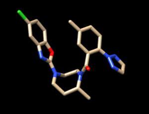
| + | #Save the structure with a new file name (i.e. 4s0v_ligand_only.pdb). The image will look similar to this: | ||
| + | [[File:ligandonly.png|thumb|center]] | ||
| + | Before we start preparing the ligand for docking we need to again save a .mol2 file for the structure in this state. Go to File → Save Mol2 and give the file a descriptive name such as 4s0v_no_hydrogens_no_charges.mol2 | ||
| − | + | Once we have the ligand saved as its own file we follow the same two steps we did for the protein: | |
| + | #Add hydrogens | ||
| + | #Add charges | ||
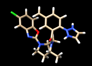
| + | These steps are a bit more complicated for the ligand because Chimera may have mistakes and we need to do our best to determine where hydrogens should be, what the overall charge of the ligand is, and what changes we need to make to the results presented by Chimera. Once the hydrogens are added to the ligand your file should be similar to: | ||
| + | |||
| + | [[File: hydrogensafter.png|thumb|center]] | ||
| + | |||
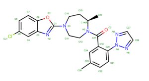
| + | To determine if Chimera added hydrogens to the correct location we should look at the 2D structure of the ligand. This can be found on the pdb page where we downloaded the .pdb file. | ||
| + | [[File: 2Dligand.png|center]] | ||
| + | |||
| + | clicking on the 2D image of the ligand brings up an enlarged image: | ||
| + | [[File: ligandlayout.png|thumb|center]] | ||
| + | |||
| + | Another useful tip is to google the compound name of the ligand to try and find structures of it to compare against. | ||
| + | |||
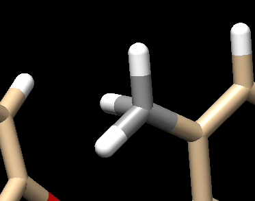
| + | Once you have these two references, you'll want to start with the carbon atoms. We see on C29 there are 2 hydrogens but this should really be a methyl group (3 hydrogens). To fix this: | ||
| + | *select both hydrogens bonded to C29 | ||
| + | *Actions → Atom/Bonds → Delete | ||
| + | *Select the carbon atom from which you just deleted the two hydrogens | ||
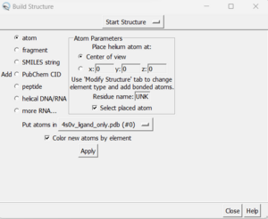
| + | *Tools → Structure Editing → Build Structure (the following dialogue box will appear): | ||
| + | [[File: buildstructure.png|thumb|center]] | ||
| + | *In the top drop down, change from 'Start Structure' to 'Modify Structure' | ||
| + | *Ensure the element says 'C' for carbon, and choose 4 bonds (since we want this carbon to have three hydrogens as opposed to the 2 hydrogens that Chimera gave it). | ||
| + | *Click 'Apply' | ||
| + | |||
| + | Your structure should now show a methyl group: | ||
| + | [[File: methyl.png|center]] | ||
| + | |||
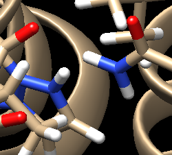
| + | Next look at the oxygen atoms and do the same thing in determining if the protonation state of each is correct. For this structure it is, so we can move onto examining the nitrogen atoms. This is a bit trickier and it's not always obvious what the protonation state should be. A good way to determine this is to look at the original pdb file, with both the ligand and protein, with hydrogens added and determine if there are any interactions that don't seems right. To do this: | ||
| + | *Close your current session | ||
| + | *Open the original pdb that was downloaded | ||
| + | *Add hydrogens following the steps outlines above | ||
| + | *Look for interactions | ||
| + | |||
| + | Automatic protonation resulted in the addition of two hydrogens to one of the rings where, in the structure of the lone compound, the adjacent nitrogens form double bonds with surrounding carbons and are not bound to hydrogen atoms. Removing these two hydrogens preserves the native structure of the compound. | ||
| + | [[File: Hydrogenint.png|center]] | ||
| + | |||
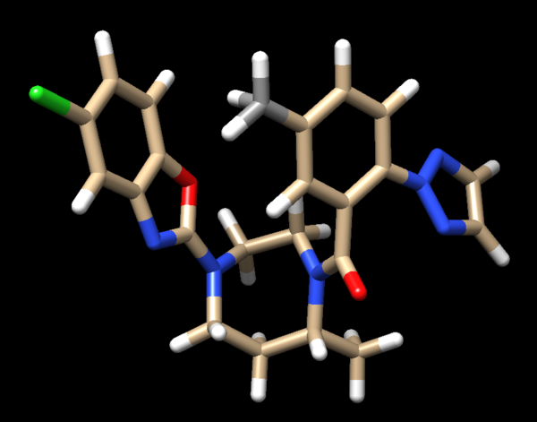
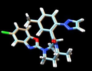
| + | Looking at the ligand further we determined that the second hydrogen on the opposite nitrogen also didn't belong so that one was also removed. This is the final change we need to make to the ligand structure which now looks like this: | ||
| + | [[File: finalligand.png|center|600px]] | ||
| + | |||
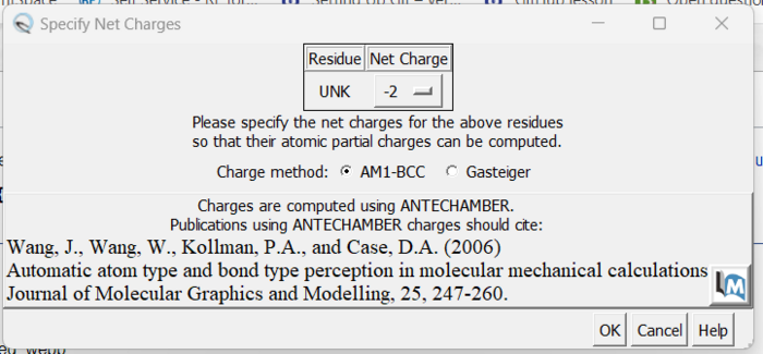
| + | The final step is to add charges to the ligand. We follow the same steps as for the protein except after the dialogue box appear and we click 'OK', a second box will appear: | ||
| + | [[File: chargeboxes.png|center|700px]] | ||
| + | |||
| + | Here a knowledge of organic chemistry will be needed. Chimera sees that we removed two hydrogens so expects the ligand charge to be -2 but the overall charge of the ligand should be 0. Simply make this change in the drop down and click 'OK'. When the program is completed, you see the total charge calculated for the ligand in the lower left hand corner. This number should be an integer (or close to it). We are now done prep'ing the ligand for docking. | ||
| + | |||
| + | The final step is to again save two files, a .pdb and .mol2 of the structure in this state. Go to File → Save Mol2 and give the file a name such as 4s0v_ligand_hydrogens_charges.mol2 and File → Save PDB and give the file a name such as 4s0v_ligand_hydrogens_charges.pdb. | ||
| + | |||
| + | ===Final Steps=== | ||
| + | Before moving onto finding the binding site of the protein we need to move the four .mol2 files over to Seawulf. Do this using the following scp command: | ||
| + | scp *.mol2 username@login.seawulf.stonybrook.edu:'/gpfs/projects/AMS536/YOURYEAR/students/YOURGROUP/001.structure' | ||
=Creating the Protein Binding Site Surface= | =Creating the Protein Binding Site Surface= | ||
| + | This section will walk you through the steps necessary to identify the binding site of the protein using a function within DOCK to place surface spheres along the protein. | ||
| + | |||
===Creating the Required Surface (DMS) File=== | ===Creating the Required Surface (DMS) File=== | ||
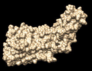
| + | In Chimera, open the 4s0v_protein_only.pdb file. Go to Actions → Surface → show. This will display the van der Waals surface of your protein. Your image should be similar to: | ||
| + | [[File: 4s0v_surface.png|thumb|center]] | ||
| + | |||
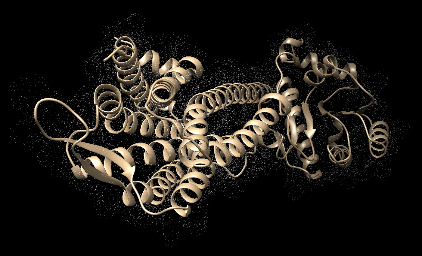
| + | Once this is done the .dms file needs to be generated by clicking on Tools → Structure Editing → Write DMS. A dialogue box will appear where you need to give the file a name, such as 4s0v_surface.dms. Once this file is saved, we need to make sure that nothing was unintended happened with DOCK during its generation. We do this by overlaying the .dms file with the protein_only file. To do this, close your current session, open the 4s0v_protein_only.pdb and then open the 4s0v_surface.dms. If everything worked as it should you should see an image similar to: | ||
| + | [[File: Dms_overlay.png|center]] | ||
| + | |||
| + | As you can see, the small dots (which is the .dms file) is perfectly aligned over the protein structure. Now that we have verified that everything looks good, we can continue. | ||
===Generating Spheres for the Binding Site=== | ===Generating Spheres for the Binding Site=== | ||
| + | Now that we have a .dms file, we need to find the binding site of the protein using a DOCK program called sphgen. This program is run on the command line on Seawulf. In order for it to run properly you need to scp the .dms file to the 002.surface_spheres directory using the command: | ||
| + | scp filename.dms username@login.seawulf.stonybrook.edu:'/gpfs/projects/AMS536/YOURYEAR/students/YOURGROUP/002.surface_spheres' | ||
| − | + | Once the file is in your 002.surface_spheres directory you need to create a file to run sphgen. Type: | |
| + | vi INSPH | ||
| − | = | + | this will open a new text document with the name INSPH. Put the following in the document replacing the filenames with your specific files: |
| + | 4s0v_surface.dms | ||
| + | R | ||
| + | X | ||
| + | 0.0 | ||
| + | 4.0 | ||
| + | 1.4 | ||
| + | 4s0v_binding_spheres.sph | ||
| + | |||
| + | Note that the first and last lines need to be updated to be the name of your files. Save this file and return to the command line using the command: | ||
| + | sphgen -i INSPH -o OUTSPH | ||
| + | |||
| + | When this is completed you will see the 4sv0_binding_spheres.sph in your directory. Once again we need to verify that this file was generated properly. Do this by comparing it to the original .pdb. Using scp, move the output file (in this case 4s0v_binding_spheres.sph) back to your local computer and open the file in a new Chimera session. In the same session, open the original .pdb file and the two structures should be aligned to each other. Your image should be similar to: | ||
| + | [[File: Spheres_and_original.png|thumb|center]] | ||
| + | |||
| + | As you can see, the ribbon of the original file is aligned to the spheres we just generated. At this point we can move onto the next step of selecting the spheres within the binding site of the protein. | ||
| + | |||
| + | ===Binding Site Spheres=== | ||
| + | This step runs a DOCK program called sphere_selector which is again run on the command line. Log back in to Seawulf and move to your 002.surface_spheres directory. Then type: | ||
| + | sphere_selector 4s0v_binding_spheres.sph ../001.structure/4s0v_ligand_hydrogens_charges.mol2 10.0 | ||
| + | |||
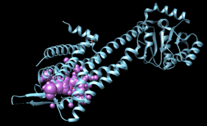
| + | When this program has successfully completed you'll see a new file in your directory called selected_spheres.sph. This file generated spheres which should line up with the binding site of the protein. We need to verify this in Chimera: | ||
| + | #scp selected_spheres.sph to your local computer | ||
| + | #Close any open sessions you have in Chimera | ||
| + | #In Chimera open selected_spheres.sph | ||
| + | #In the current session, open the original protein/ligand complex (4s0v.pdb) | ||
| + | #You should see the spheres located within the binding site of the protein, similar to: | ||
| + | |||
| + | [[File: bindingsitespheres.png|thumb|center]] | ||
| + | |||
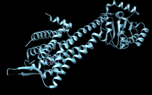
| + | While this looks good we should verify that the spheres are actually where the ligand is. Let's do this by selecting the spheres, hiding them from view, and verifying the ligand is in the same location: | ||
| + | #Hold down ctrl and click on a sphere | ||
| + | #Press the up arrow until all spheres are selected | ||
| + | #Actions → Atoms/Bonds → hide | ||
| + | #Verify the ligand is where the spheres were | ||
| + | |||
| + | [[File: withoutspheres.png|thumb|center]] | ||
| + | |||
| + | and we see the ligand is where the spheres were so we can be confident in our work so far. | ||
| + | |||
| + | =Box and Grid Generation= | ||
| + | The next step in the docking process is to generate energy interactions between the atoms of the protein and ligand. If this was done for the whole complex it would take too long to run to be useful. To get around this computationally expensive step, dock uses a box/grid method. We will define a box around the area of interest for the protein/ligand and DOCK will generate a grid within this box which will be used in the energy calculations. | ||
===Generating the Box=== | ===Generating the Box=== | ||
| + | To generate the box we will be working again on the command line using a DOCK program called showbox. Start by logging into Seawulf and navigating to your 003.gridbox directory. We need to make a new file called showbox.in by typing: | ||
| + | vi showbox.in | ||
| + | |||
| + | This will create a new file, with a filename of showbox.in and open it in vi. The following commands need to be typed: | ||
| + | Y | ||
| + | 8.0 | ||
| + | ../002.surface_spheres/selected_spheres.sph | ||
| + | 1 | ||
| + | 4s0v.box.pdb | ||
| + | |||
| + | Remember to change the last line to be a filename with the number of protein you are working with. The second line of this code (8.0) is telling dock how many angstroms from the selected spheres to draw the box. Depending on your system you may need to modify this number. | ||
| + | |||
| + | To run this file, simply type: | ||
| + | showbox < showbox.in | ||
| + | If showbox was successful the file 4s0v.box.pdb will now be in your directory. | ||
===Generating the Grid=== | ===Generating the Grid=== | ||
| + | Now that we have our box defined we need to instruct DOCK to generate the grid within it. We do this using a DOCK program called grid: | ||
| + | vi grid.in | ||
| − | = | + | This command will generate and open a file named grid.in. The commands to be typed into this file are: |
| − | === | + | allow_non_integral_charges no |
| + | compute_grids yes | ||
| + | grid_spacing 0.4 | ||
| + | output_molecule no | ||
| + | contact_score no | ||
| + | energy_score yes | ||
| + | energy_cutoff_distance 9999 | ||
| + | atom_model a | ||
| + | attractive_exponent 6 | ||
| + | repulsive_exponent 9 | ||
| + | distance_dielectric yes | ||
| + | dielectric_factor 4. | ||
| + | bump_filter yes | ||
| + | bump_overlap 0.75 | ||
| + | receptor_file ../001.structure/4s0v_protein_hydrogens_charges.mol2 | ||
| + | box_file 4s0v.box.pdb | ||
| + | vdw_definition_file /gpfs/projects/AMS536/zzz.programs/dock6.9_release/parameters/vdw_AMBER_parm99.defn | ||
| + | score_grid_prefix grid | ||
| + | |||
| + | The only change you need to make to the above commands is the receptor_file and box_file to reflect the files you previously generated. | ||
| + | |||
| + | Once this file is saved, run it: | ||
| + | grid -i grid.in -o 4s0vGridInfo.out | ||
| + | |||
| + | Be patient, this step might take a few minutes to run. You will know it's worked successfully if you see: | ||
| + | #grid.bmp | ||
| + | #grid.nrg | ||
| + | #4s0vGridInfo.out | ||
| + | |||
| + | in your directory. With the box and grid successfully generated we are ready to move onto the energy minimization step. | ||
| + | |||
| + | =Energy Minimization= | ||
| + | At its core, DOCK is finding interactions between a protein and ligand by looking at energy interactions between atoms. In order for DOCK to give the most accurate results we need to ensure that the ligand is at its lowest energy state before docking it into the binding site of the protein. | ||
| + | |||
| + | ===Ligand Minimization=== | ||
| + | For this section we will be working in the 004.energy_min directory and will be using the dock6 command. Again we need to generate the input file that dock6 needs: | ||
| + | vi min.in | ||
| + | |||
| + | Once in vi the following lines need to be typed in: | ||
| + | conformer_search_type rigid | ||
| + | use_internal_energy yes | ||
| + | internal_energy_rep_exp 12 | ||
| + | internal_energy_cutoff 100.0 | ||
| + | ligand_atom_file ../001.structure/4s0v_ligand_hydrogens_charges.mol2 | ||
| + | limit_max_ligands no | ||
| + | skip_molecule no | ||
| + | read_mol_solvation no | ||
| + | calculate_rmsd yes | ||
| + | use_rmsd_reference_mol yes | ||
| + | rmsd_reference_filename ../001.structure/4s0v_ligand_hydrogens_charges.mol2 | ||
| + | use_database_filter no | ||
| + | orient_ligand no | ||
| + | bump_filter no | ||
| + | score_molecules yes | ||
| + | contact_score_primary no | ||
| + | contact_score_secondary no | ||
| + | grid_score_primary yes | ||
| + | grid_score_secondary no | ||
| + | grid_score_rep_rad_scale 1 | ||
| + | grid_score_vdw_scale 1 | ||
| + | grid_score_es_scale 1 | ||
| + | grid_score_grid_prefix ../003.gridbox/grid | ||
| + | multigrid_score_secondary no | ||
| + | dock3.5_score_secondary no | ||
| + | continuous_score_secondary no | ||
| + | footprint_similarity_score_secondary no | ||
| + | pharmacophore_score_secondary no | ||
| + | descriptor_score_secondary no | ||
| + | gbsa_zou_score_secondary no | ||
| + | gbsa_hawkins_score_secondary no | ||
| + | SASA_score_secondary no | ||
| + | amber_score_secondary no | ||
| + | minimize_ligand yes | ||
| + | simplex_max_iterations 1000 | ||
| + | simplex_tors_premin_iterations 0 | ||
| + | simplex_max_cycles 1 | ||
| + | simplex_score_converge 0.1 | ||
| + | simplex_cycle_converge 1.0 | ||
| + | simplex_trans_step 1.0 | ||
| + | simplex_rot_step 0.1 | ||
| + | simplex_tors_step 10.0 | ||
| + | simplex_random_seed 0 | ||
| + | simplex_restraint_min yes | ||
| + | simplex_coefficient_restraint 10.0 | ||
| + | atom_model all | ||
| + | vdw_defn_file /gpfs/projects/AMS536/zzz.programs/dock6.9_release/parameters/vdw_AMBER_parm99.defn | ||
| + | flex_defn_file /gpfs/projects/AMS536/zzz.programs/dock6.9_release/parameters/flex.defn | ||
| + | flex_drive_file /gpfs/projects/AMS536/zzz.programs/dock6.9_release/parameters/flex_drive.tbl | ||
| + | ligand_outfile_prefix 4s0v.lig.min | ||
| + | write_orientations no | ||
| + | num_scored_conformers 1 | ||
| + | rank_ligands no | ||
| + | |||
| + | And the file is run with the following command: | ||
| + | dock6 -i min.in -o min.out | ||
| + | |||
| + | After successful completion of the program two new files will be in your directory: | ||
| + | *min.out | ||
| + | *4s0v.lig.min.mol2 | ||
| + | |||
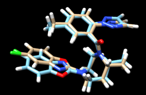
| + | scp the .mol2 file back to your local computer. To view the changes that dock made to the structure, and open the 4s0v.lig.min.mol2 file in Chimera and in the same session, open the 4s0v_ligand_with_chareg.pdb file. Remember the 4s0v_ligand_with_charge.pdb is the file we saved after making the protonation changes to the ligand. You should see something similar to: | ||
| + | [[File: ligandminimized.png|thumb|center]] | ||
| + | |||
| + | And you can see DOCK has made small changes to the ligand structure. | ||
=== Footprint Analysis=== | === Footprint Analysis=== | ||
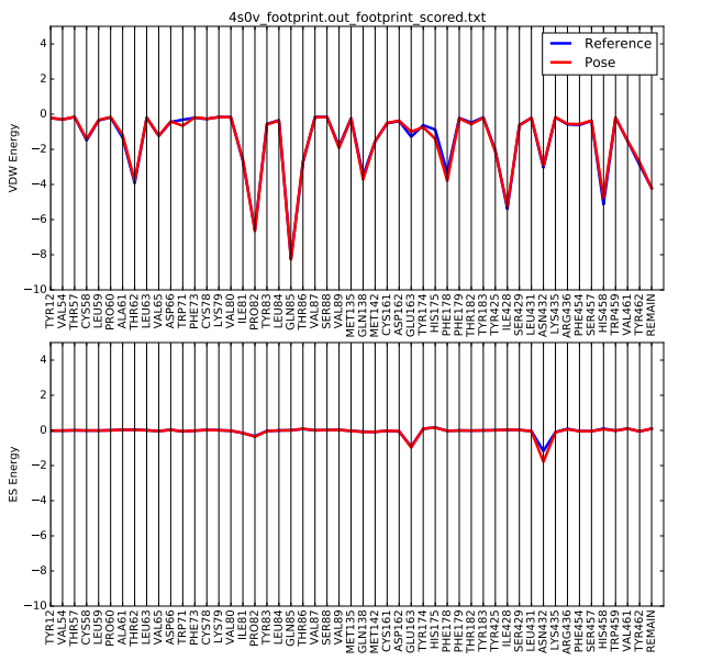
| + | At its core, DOCK can be thought of as a program which evaluates, minimizes, and uses the electrostatic and VDW interactions between the ligand and protein to determine how they bind to each other. A footprint analysis is a way to visualize these interactions and possibly be used to design new ligands with the same, or better, set of energetics. The steps in this section will be done on Seawulf in the 005.footprint directory. We will be using the dock6 command and again need to create an input file: | ||
| + | vi footprint.in | ||
| + | The following lines needed to be typed into the newly created file: | ||
| + | conformer_search_type rigid | ||
| + | use_internal_energy no | ||
| + | ligand_atom_file ../004.energy_min/4s0v.lig.min_scored.mol2 | ||
| + | limit_max_ligands no | ||
| + | skip_molecule no | ||
| + | read_mol_solvation no | ||
| + | calculate_rmsd no | ||
| + | use_database_filter no | ||
| + | orient_ligand no | ||
| + | bump_filter no | ||
| + | score_molecules yes | ||
| + | contact_score_primary no | ||
| + | contact_score_secondary no | ||
| + | grid_score_primary no | ||
| + | grid_score_secondary no | ||
| + | multigrid_score_primary no | ||
| + | multigrid_score_secondary no | ||
| + | dock3.5_score_primary no | ||
| + | dock3.5_score_secondary no | ||
| + | continuous_score_primary no | ||
| + | continuous_score_secondary no | ||
| + | footprint_similarity_score_primary yes | ||
| + | footprint_similarity_score_secondary no | ||
| + | fps_score_use_footprint_reference_mol2 yes | ||
| + | fps_score_footprint_reference_mol2_filename ../001.structure/4s0v_ligand_hydrogens_charges.mol2 | ||
| + | fps_score_foot_compare_type Euclidean | ||
| + | fps_score_normalize_foot no | ||
| + | fps_score_foot_comp_all_residue yes | ||
| + | fps_score_receptor_filename ../001.structure/4s0v_protein_hydrogens_charges.mol2 | ||
| + | fps_score_vdw_att_exp 6 | ||
| + | fps_score_vdw_rep_exp 9 | ||
| + | fps_score_vdw_rep_rad_scale 1 | ||
| + | fps_score_use_distance_dependent_dielectric yes | ||
| + | fps_score_dielectric 4.0 | ||
| + | fps_score_vdw_fp_scale 1 | ||
| + | fps_score_es_fp_scale 1 | ||
| + | fps_score_hb_fp_scale 0 | ||
| + | pharmacophore_score_secondary no | ||
| + | descriptor_score_secondary no | ||
| + | gbsa_zou_score_secondary no | ||
| + | gbsa_hawkins_score_secondary no | ||
| + | SASA_score_secondary no | ||
| + | amber_score_secondary no | ||
| + | minimize_ligand no | ||
| + | atom_model all | ||
| + | vdw_defn_file /gpfs/projects/AMS536/zzz.programs/dock6.9_release/parameters/vdw_AMBER_parm99.defn | ||
| + | flex_defn_file /gpfs/projects/AMS536/zzz.programs/dock6.9_release/parameters/flex.defn | ||
| + | flex_drive_file /gpfs/projects/AMS536/zzz.programs/dock6.9_release/parameters/flex_drive.tbl | ||
| + | ligand_outfile_prefix 4s0v_footprint.out | ||
| + | write_footprints yes | ||
| + | write_hbonds yes | ||
| + | write_orientations no | ||
| + | num_scored_conformers 1 | ||
| + | rank_ligands no | ||
| + | to generate the footprint of the ligand/protein interaction type: | ||
| + | dock6 -i footprint.in | ||
| + | |||
| + | Again, you will know the program successfully ran if the following three files are now in your directory: | ||
| + | *4s0v_footprint.out_footprint_scored.txt | ||
| + | *4s0v_footprint.out_hbond_scored.txt | ||
| + | *4s0v_footprint.out_scored.mol2 | ||
| + | |||
| + | In order to view/analyze these results we need to use a python script that is located in the class directory. Copy it over to your 005.footprint directory with the following command: | ||
| + | cp /gpfs/projects/AMS536/2020/536_class/steve_ta/footprint_test_1.21.2020/plot_footprint_single_magnitude.py . | ||
| + | |||
| + | To run this script type: | ||
| + | python plot_footprint_single_magnitude.py 4s0v_footprint.out_footprint_scored.txt 50 | ||
| + | |||
| + | If you get an error when running this script you may need to load a module in order to access python. Try typing: | ||
| + | module load anaconda/2 | ||
| + | |||
| + | and then re-running the python script. It should work now. | ||
| + | |||
| + | Once the script is completed you will see a .pdf file in your directory. scp this file back to your local computer. The file contains two plots that shows the energetic signature for the 50 most significant residues and will look similar to: | ||
| + | [[File: 4s0v_footprint.png|center]] | ||
| + | |||
| + | =DOCK= | ||
| + | We will be exploring three different options of the DOCK program: | ||
| + | #Rigid Docking | ||
| + | #Fixed Anchor Docking | ||
| + | #Flexible Docking | ||
| + | |||
| + | Each option has it's own pros and cons and your individual system should dictate which option you choose. Note: In the input file for each of these options has a line: | ||
| + | num_scored_conformers 1 | ||
| + | |||
| + | Changing this number will change the number of conformations saved from the docking session. | ||
===Rigid Docking=== | ===Rigid Docking=== | ||
| + | When using rigid docking, the DOCK program does not sample different conformations of the ligand to try and find the most energetically stable. It simply treats the ligand as a rigid structure and tries to fit it into the binding site of the protein. For this step we will be using the energy minimized ligand file we generated above. This section will again be completed on Seawulf, please move to the 006.rigid_docking directory. | ||
| + | |||
| + | Again we need an input file that can be created using the command: | ||
| + | vi rigid.in | ||
| + | |||
| + | The following lines need to be typed into the file: | ||
| + | conformer_search_type rigid | ||
| + | write_fragment_libraries no | ||
| + | user_specified_anchor no | ||
| + | limit_max_anchors no | ||
| + | min_anchor_size 5 | ||
| + | pruning_use_clustering yes | ||
| + | pruning_max_orients 1000 | ||
| + | pruning_clustering_cutoff 100 | ||
| + | pruning_conformer_score_cutoff 100.0 | ||
| + | pruning_conformer_score_scaling_factor 1.0 | ||
| + | use_clash_overlap no | ||
| + | write_growth_tree no | ||
| + | use_internal_energy yes | ||
| + | internal_energy_rep_exp 12 | ||
| + | internal_energy_cutoff 100.0 | ||
| + | ligand_atom_file ../004.energy_min/4s0v.lig.min_scored.mol2 | ||
| + | limit_max_ligands no | ||
| + | skip_molecule no | ||
| + | read_mol_solvation no | ||
| + | calculate_rmsd yes | ||
| + | use_rmsd_reference_mol yes | ||
| + | rmsd_reference_filename ../004.energy_min/4s0v.lig.min_scored.mol2 | ||
| + | use_database_filter no | ||
| + | orient_ligand yes | ||
| + | automated_matching yes | ||
| + | receptor_site_file ../002.surface_spheres/selected_spheres.sph | ||
| + | max_orientations 1000 | ||
| + | critical_points no | ||
| + | chemical_matching no | ||
| + | use_ligand_spheres no | ||
| + | bump_filter no | ||
| + | score_molecules yes | ||
| + | contact_score_primary no | ||
| + | contact_score_secondary no | ||
| + | grid_score_primary yes | ||
| + | grid_score_secondary no | ||
| + | grid_score_rep_rad_scale 1 | ||
| + | grid_score_vdw_scale 1 | ||
| + | grid_score_es_scale 1 | ||
| + | grid_score_grid_prefix ../003.gridbox/grid | ||
| + | multigrid_score_secondary no | ||
| + | dock3.5_score_secondary no | ||
| + | continuous_score_secondary no | ||
| + | footprint_similarity_score_secondary no | ||
| + | pharmacophore_score_secondary no | ||
| + | descriptor_score_secondary no | ||
| + | gbsa_zou_score_secondary no | ||
| + | gbsa_hawkins_score_secondary no | ||
| + | SASA_score_secondary no | ||
| + | amber_score_secondary no | ||
| + | minimize_ligand yes | ||
| + | minimize_anchor yes | ||
| + | minimize_flexible_growth yes | ||
| + | use_advanced_simplex_parameters no | ||
| + | simplex_max_cycles 1 | ||
| + | simplex_score_converge 0.1 | ||
| + | simplex_cycle_converge 1.0 | ||
| + | simplex_trans_step 1.0 | ||
| + | simplex_rot_step 0.1 | ||
| + | simplex_tors_step 10.0 | ||
| + | simplex_anchor_max_iterations 500 | ||
| + | simplex_grow_max_iterations 500 | ||
| + | simplex_grow_tors_premin_iterations 0 | ||
| + | simplex_random_seed 0 | ||
| + | simplex_restraint_min no | ||
| + | atom_model all | ||
| + | vdw_defn_file /gpfs/projects/AMS536/zzz.programs/dock6.9_release/parameters/vdw_AMBER_parm99.defn | ||
| + | flex_defn_file /gpfs/projects/AMS536/zzz.programs/dock6.9_release/parameters/flex.defn | ||
| + | flex_drive_file /gpfs/projects/AMS536/zzz.programs/dock6.9_release/parameters/flex_drive.tbl | ||
| + | ligand_outfile_prefix rigid.out | ||
| + | write_orientations no | ||
| + | num_scored_conformers 1 | ||
| + | rank_ligands no | ||
| + | |||
| + | Remember to again change the necessary lines to point to your specific files. Once this is completed run the program by typing: | ||
| + | dock6 -i rigid.in -o rigid.out | ||
| + | |||
| + | Again, be patient as this may take a few minutes to complete. Once it's done running you will see two new files in your directory: | ||
| + | *rigid.out_scored.mol2 | ||
| + | *rigid.out | ||
| + | |||
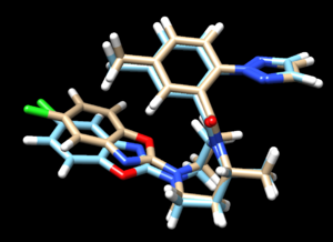
| + | scp the .mol2 file over to your local computer. Start a new session in Chimera and open the energy minimized ligand file from the previous step and the rigid docked ligand you just created (4s0v.lig.min_scored.mol2 and rigid.out_scored.mol2) to view the differences between the energy minimized ligand and DOCK's attempt to rigid dock that structure into the protein. | ||
| + | |||
| + | [[File: rigidoverlay.png|thumb|center]] | ||
| + | |||
| + | Looking at this file we see that the two are very similar to each other. | ||
| + | |||
| + | Now we can look at the other file that dock generated, rigid.out. If we scroll to the bottom you will see grid scoring for this run: | ||
| + | [[File: Ridiggridscore.png|center]] | ||
===Fixed Anchor Docking=== | ===Fixed Anchor Docking=== | ||
| + | The next DOCK option we will be looking at is called 'Fixed Anchor Docking'. For this option, DOCK cuts the ligand into fragments along its rotatable bonds. It then chooses the largest fragment as the 'anchor' and orients this fragment into the binding site of the protein. Once this is completed, the next fragments are added to the ligand, orientating them such that their energy is minimized but keeping them as rigid bodies. Comparing this to Rigid Docking, we see that more conformational sampling is being done but still within limits since each fragment is considered rigid. | ||
| + | |||
| + | We'll be working on the command line again, please move to the 007.fixed_anchor_docking directory and create an input file called fixed.in: | ||
| + | vi fixed.in | ||
| + | |||
| + | and type the following lines: | ||
| + | conformer_search_type flex | ||
| + | write_fragment_libraries no | ||
| + | user_specified_anchor no | ||
| + | limit_max_anchors no | ||
| + | min_anchor_size 5 | ||
| + | pruning_use_clustering yes | ||
| + | pruning_max_orients 1000 | ||
| + | pruning_clustering_cutoff 100 | ||
| + | pruning_conformer_score_cutoff 100.0 | ||
| + | pruning_conformer_score_scaling_factor 1.0 | ||
| + | use_clash_overlap no | ||
| + | write_growth_tree no | ||
| + | use_internal_energy yes | ||
| + | internal_energy_rep_exp 12 | ||
| + | internal_energy_cutoff 100.0 | ||
| + | ligand_atom_file ../004.energy_min/4s0v.lig.min_scored.mol2 | ||
| + | limit_max_ligands no | ||
| + | skip_molecule no | ||
| + | read_mol_solvation no | ||
| + | calculate_rmsd yes | ||
| + | use_rmsd_reference_mol yes | ||
| + | rmsd_reference_filename ../004.energy_min/4s0v.lig.min_scored.mol2 | ||
| + | use_database_filter no | ||
| + | orient_ligand no | ||
| + | bump_filter no | ||
| + | score_molecules yes | ||
| + | contact_score_primary no | ||
| + | contact_score_secondary no | ||
| + | grid_score_primary yes | ||
| + | grid_score_secondary no | ||
| + | grid_score_rep_rad_scale 1 | ||
| + | grid_score_vdw_scale 1 | ||
| + | grid_score_es_scale 1 | ||
| + | grid_score_grid_prefix ../003.gridbox/grid | ||
| + | multigrid_score_secondary no | ||
| + | dock3.5_score_secondary no | ||
| + | continuous_score_secondary no | ||
| + | footprint_similarity_score_secondary no | ||
| + | pharmacophore_score_secondary no | ||
| + | descriptor_score_secondary no | ||
| + | gbsa_zou_score_secondary no | ||
| + | gbsa_hawkins_score_secondary no | ||
| + | SASA_score_secondary no | ||
| + | amber_score_secondary no | ||
| + | minimize_ligand yes | ||
| + | minimize_anchor yes | ||
| + | minimize_flexible_growth yes | ||
| + | use_advanced_simplex_parameters no | ||
| + | simplex_max_cycles 1 | ||
| + | simplex_score_converge 0.1 | ||
| + | simplex_cycle_converge 1 | ||
| + | simplex_trans_step 1 | ||
| + | simplex_rot_step 0.1 | ||
| + | simplex_tors_step 10.0 | ||
| + | simplex_anchor_max_iterations 500 | ||
| + | simplex_grow_max_iterations 500 | ||
| + | simplex_grow_tors_premin_iterations 0 | ||
| + | simplex_random_seed 0 | ||
| + | simplex_restraint_min no | ||
| + | atom_model all | ||
| + | vdw_defn_file /gpfs/projects/AMS536/zzz.programs/dock6.9_release/parameters/vdw_AMBER_parm99.defn | ||
| + | flex_defn_file /gpfs/projects/AMS536/zzz.programs/dock6.9_release/parameters/flex.defn | ||
| + | flex_drive_file /gpfs/projects/AMS536/zzz.programs/dock6.9_release/parameters/flex_drive.tbl | ||
| + | ligand_outfile_prefix 4s0v_fixed_output | ||
| + | write_orientations no | ||
| + | num_scored_conformers 1 | ||
| + | rank_ligands no | ||
| + | |||
| + | Again, change the necessary lines to point to your specific files. To run this file type: | ||
| + | dock6 -i fixed.in -o fixed.out | ||
| + | |||
| + | Once it's done running you will see two new files in your directory: | ||
| + | *fixed.out | ||
| + | *4s0v_fixed_output_scored.mol2 | ||
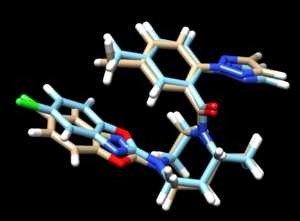
| + | scp the .mol2 file over to your local computer. Start a new session in Chimera and open the energy minimized ligand file from the previous step and the fixed anchor docked ligand you just created (4s0v.lig.min_scored.mol2 and 4s0v_fixed_output_scored.mol2) to view the differences between the energy minimized ligand and DOCK's attempt to place that structure using its fixed anchor algorithm. Your image should be similar to: | ||
| + | |||
| + | [[File: fixedoverlay.png|thumb|center]] | ||
| + | |||
| + | And looking at the grid score in fixed.out we see: | ||
| + | |||
| + | [[File: fixedscore.png|thumb|center]] | ||
| + | |||
| + | Let's now open both .mol2 files in Chimera and see how they compare to each other: | ||
| + | |||
| + | [[File: rigidvsfixed.png|thumb|center]] | ||
| + | Doing this allows us to see the differences in the poses of the two different docking methods. | ||
===Flexible Docking=== | ===Flexible Docking=== | ||
| + | The final docking method we're going to look at is called flexible docking. This is the most computationally expensive of the three methods, because now DOCK will sample all conformations of all rotatable bonds within the ligand attempting to minimize the energetics of the ligand. Once again we will be working on the command line in Seawulf, but now in your 008.flex_docking directory. | ||
| + | |||
| + | Create your input file: | ||
| + | vi flex.in | ||
| + | |||
| + | And type the following lines into your input file: | ||
| + | |||
| + | conformer_search_type flex | ||
| + | write_fragment_libraries no | ||
| + | user_specified_anchor no | ||
| + | limit_max_anchors no | ||
| + | min_anchor_size 5 | ||
| + | pruning_use_clustering yes | ||
| + | pruning_max_orients 1000 | ||
| + | pruning_clustering_cutoff 100 | ||
| + | pruning_conformer_score_cutoff 100.0 | ||
| + | pruning_conformer_score_scaling_factor 1.0 | ||
| + | use_clash_overlap no | ||
| + | write_growth_tree no | ||
| + | use_internal_energy yes | ||
| + | internal_energy_rep_exp 12 | ||
| + | internal_energy_cutoff 100.0 | ||
| + | ligand_atom_file ../004.energy_min/4s0v.lig.min_scored.mol2 | ||
| + | limit_max_ligands no | ||
| + | skip_molecule no | ||
| + | read_mol_solvation no | ||
| + | calculate_rmsd yes | ||
| + | use_rmsd_reference_mol yes | ||
| + | rmsd_reference_filename ../004.energy_min/4s0v.lig.min_scored.mol2 | ||
| + | use_database_filter no | ||
| + | orient_ligand yes | ||
| + | automated_matching yes | ||
| + | receptor_site_file ../002.surface_spheres/selected_spheres.sph | ||
| + | max_orientations 1000 | ||
| + | critical_points no | ||
| + | chemical_matching no | ||
| + | use_ligand_spheres no | ||
| + | bump_filter no | ||
| + | score_molecules yes | ||
| + | contact_score_primary no | ||
| + | contact_score_secondary no | ||
| + | grid_score_primary yes | ||
| + | grid_score_secondary no | ||
| + | grid_score_rep_rad_scale 1 | ||
| + | grid_score_vdw_scale 1 | ||
| + | grid_score_es_scale 1 | ||
| + | grid_score_grid_prefix ../003.gridbox/grid | ||
| + | multigrid_score_secondary no | ||
| + | dock3.5_score_secondary no | ||
| + | continuous_score_secondary no | ||
| + | footprint_similarity_score_secondary no | ||
| + | pharmacophore_score_secondary no | ||
| + | descriptor_score_secondary no | ||
| + | gbsa_zou_score_secondary no | ||
| + | gbsa_hawkins_score_secondary no | ||
| + | SASA_score_secondary no | ||
| + | amber_score_secondary no | ||
| + | minimize_ligand yes | ||
| + | minimize_anchor yes | ||
| + | minimize_flexible_growth yes | ||
| + | use_advanced_simplex_parameters no | ||
| + | simplex_max_cycles 1 | ||
| + | simplex_score_converge 0.1 | ||
| + | simplex_cycle_converge 1.0 | ||
| + | simplex_trans_step 1.0 | ||
| + | simplex_rot_step 0.1 | ||
| + | simplex_tors_step 10.0 | ||
| + | simplex_anchor_max_iterations 500 | ||
| + | simplex_grow_max_iterations 500 | ||
| + | simplex_grow_tors_premin_iterations 0 | ||
| + | simplex_random_seed 0 | ||
| + | simplex_restraint_min no | ||
| + | atom_model all | ||
| + | vdw_defn_file /gpfs/projects/AMS536/zzz.programs/dock6.9_release/parameters/vdw_AMBER_parm99.defn | ||
| + | flex_defn_file /gpfs/projects/AMS536/zzz.programs/dock6.9_release/parameters/flex.defn | ||
| + | flex_drive_file /gpfs/projects/AMS536/zzz.programs/dock6.9_release/parameters/flex_drive.tbl | ||
| + | ligand_outfile_prefix flex.out | ||
| + | write_orientations no | ||
| + | num_scored_conformers 1 | ||
| + | rank_ligands no | ||
| + | |||
| + | and run the file using the command: | ||
| + | dock6 -i flex.in -o flex.out | ||
| + | |||
| + | When the program has finished running you will see two new files in your directory: | ||
| + | *flex.out | ||
| + | *flex.out_scored.mol2 | ||
| + | |||
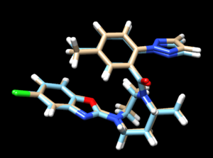
| + | again, scp the .mol2 file to your local computer and open it into a new session in Chimera. Overlaying this file with the energy minimized ligand we see: | ||
| + | [[File: flexoverlay.png|thumb|center]] | ||
| + | |||
| + | Looking at the grid scores from flex.out: | ||
| + | |||
| + | [[File: flexgridscore.png|thumb|center]] | ||
| + | |||
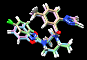
| + | Its interesting to now load the results from all three docking methods, along with the energy minimized ligand, and see the differences: | ||
| + | |||
| + | [[File: fouroverlays.png|thumb|center]] | ||
| + | |||
| + | In this image: | ||
| + | *tan is rigid docking | ||
| + | *green is the energy minimized ligand | ||
| + | *blue is the flexible docking | ||
| + | *pink is the fixed anchor docking | ||
| + | |||
| + | = Virtual Screening of a Ligand Library = | ||
| + | Up to this point we have been docking one molecule, the ligand that was in the protein/ligand complex from the pdb. But DOCK has the ability to find interactions between the protein and many different small molecules, finding the top binding ligands. This allows us to "screen" thousands of molecules but only spend time digging into the details of the top results. For this tutorial, we have created a file, VS_library_5K.mol2, which contains all the information needed on the molecules we wish to screen. Again we will be working on the command line in the 009.virtual_screening directory. | ||
| + | |||
| + | Let's create our input file: | ||
| + | vi virtual.in | ||
| + | |||
| + | which needs to have the following lines typed in: | ||
| + | conformer_search_type flex | ||
| + | write_fragment_libraries no | ||
| + | user_specified_anchor no | ||
| + | limit_max_anchors no | ||
| + | min_anchor_size 5 | ||
| + | pruning_use_clustering yes | ||
| + | pruning_max_orients 1000 | ||
| + | pruning_clustering_cutoff 100 | ||
| + | pruning_conformer_score_cutoff 100.0 | ||
| + | pruning_conformer_score_scaling_factor 1.0 | ||
| + | use_clash_overlap no | ||
| + | write_growth_tree no | ||
| + | use_internal_energy yes | ||
| + | internal_energy_rep_exp 9 | ||
| + | internal_energy_cutoff 100.0 | ||
| + | ligand_atom_file /gpfs/projects/AMS536/zzz.programs/VS_library_5K.mol2 | ||
| + | limit_max_ligands no | ||
| + | skip_molecule no | ||
| + | read_mol_solvation no | ||
| + | calculate_rmsd no | ||
| + | use_database_filter no | ||
| + | orient_ligand yes | ||
| + | automated_matching yes | ||
| + | receptor_site_file ../002.surface_spheres/selected_spheres.sph | ||
| + | max_orientations 1000 | ||
| + | critical_points no | ||
| + | chemical_matching no | ||
| + | use_ligand_spheres no | ||
| + | bump_filter no | ||
| + | score_molecules yes | ||
| + | contact_score_primary no | ||
| + | contact_score_secondary no | ||
| + | grid_score_primary yes | ||
| + | grid_score_secondary no | ||
| + | grid_score_rep_rad_scale 1 | ||
| + | grid_score_vdw_scale 1 | ||
| + | grid_score_es_scale 1 | ||
| + | grid_score_grid_prefix ../003.gridbox/grid | ||
| + | multigrid_score_secondary no | ||
| + | dock3.5_score_secondary no | ||
| + | continuous_score_secondary no | ||
| + | footprint_similarity_score_secondary no | ||
| + | pharmacophore_score_secondary no | ||
| + | descriptor_score_secondary no | ||
| + | gbsa_zou_score_secondary no | ||
| + | gbsa_hawkins_score_secondary no | ||
| + | SASA_score_secondary no | ||
| + | amber_score_secondary no | ||
| + | minimize_ligand yes | ||
| + | minimize_anchor yes | ||
| + | minimize_flexible_growth yes | ||
| + | use_advanced_simplex_parameters no | ||
| + | simplex_max_cycles 1 | ||
| + | simplex_score_converge 0.1 | ||
| + | simplex_cycle_converge 1.0 | ||
| + | simplex_trans_step 1.0 | ||
| + | simplex_rot_step 0.1 | ||
| + | simplex_tors_step 10.0 | ||
| + | simplex_anchor_max_iterations 500 | ||
| + | simplex_grow_max_iterations 500 | ||
| + | simplex_grow_tors_premin_iterations 0 | ||
| + | simplex_random_seed 0 | ||
| + | simplex_restraint_min no | ||
| + | atom_model all | ||
| + | vdw_defn_file /gpfs/projects/AMS536/zzz.programs/dock6.9_release/parameters/vdw_AMBER_parm99.defn | ||
| + | flex_defn_file /gpfs/projects/AMS536/zzz.programs/dock6.9_release/parameters/flex.defn | ||
| + | flex_drive_file /gpfs/projects/AMS536/zzz.programs/dock6.9_release/parameters/flex_drive.tbl | ||
| + | ligand_outfile_prefix virtual.out | ||
| + | write_orientations no | ||
| + | num_scored_conformers 1 | ||
| + | rank_ligands no | ||
| + | |||
| + | Running DOCK on 5000 molecules CANNOT be done on the login node of Seawulf. You will crash the system and have your login information suspended. All computationally intensive jobs such as this need to be submitted to Seawulf using the scheduler, Slurm. To do this you need to create a slurm script, which is just a text file that tells Seawulf what you want to run. | ||
| + | |||
| + | Create your slurm script | ||
| + | vi 4s0v_virtual.slurm | ||
| + | |||
| + | The contents of the slurm script are: | ||
| + | #!/bin/bash | ||
| + | # | ||
| + | #SBATCH --job-name=4s0v_vs_tutorial | ||
| + | #SBATCH --output=vs_output.txt | ||
| + | #SBATCH --ntasks=24 | ||
| + | #SBATCH --nodes=6 | ||
| + | #SBATCH --time=48:00:00 | ||
| + | #SBATCH -p long-24core | ||
| + | |||
| + | module load intel/mpi/64/2018/18.0.3 | ||
| + | |||
| + | mpirun -np 144 dock6.mpi -i virtual.in -o virtual.out | ||
| + | |||
| + | To get this script to run, on the command line, type: | ||
| + | module load slurm | ||
| + | sbatch 4s0v_virtual.slurm | ||
| + | |||
| + | This script is virtually screening 5,000 molecules and could take up to 48 hours to complete. After 48 hours, slurm will stop the job even if all 5,000 compounds haven't been docked yet. At any point while it's running, if you want to see how many molecules have been docked so far, simply type: | ||
| + | grep Molecule: virtual.out | wc -l | ||
| + | |||
| + | be sure to type the above command from your 009.virtual_screening directory. | ||
| + | |||
| + | After 48 hours, our script stopped running and 4549 molecules had been docked to our protein. In order to find the top "hits" of small molecules we need to minimize the outputs which is outlined in the next section. | ||
| + | |||
| + | =Cartesian Minimization of Virtually Screened Small Molecules= | ||
| + | In order to minimize the 4549 molecules that were docked we need to create an input file. cd over to your 010.cartesian_minimization directory and create the input file: | ||
| + | vi min.in | ||
| + | |||
| + | and type in the following lines: | ||
| + | conformer_search_type rigid | ||
| + | use_internal_energy yes | ||
| + | internal_energy_rep_exp 12 | ||
| + | internal_energy_cutoff 100 | ||
| + | ligand_atom_file ../009.virtual_screening/virtual.out_scored.mol2 | ||
| + | limit_max_ligands no | ||
| + | skip_molecule no | ||
| + | read_mol_solvation no | ||
| + | calculate_rmsd no | ||
| + | use_database_filter no | ||
| + | orient_ligand no | ||
| + | bump_filter no | ||
| + | score_molecules yes | ||
| + | contact_score_primary no | ||
| + | contact_score_secondary no | ||
| + | grid_score_primary no | ||
| + | grid_score_secondary no | ||
| + | multigrid_score_primary no | ||
| + | multigrid_score_secondary no | ||
| + | dock3.5_score_primary no | ||
| + | dock3.5_score_secondary no | ||
| + | continuous_score_primary yes | ||
| + | continuous_score_secondary no | ||
| + | cont_score_rec_filename ../001.structure/4s0v_protein_hydrogens_charges.mol2 | ||
| + | cont_score_att_exp 6 | ||
| + | cont_score_rep_exp 12 | ||
| + | cont_score_rep_rad_scale 1 | ||
| + | cont_score_use_dist_dep_dielectric yes | ||
| + | cont_score_dielectric 4.0 | ||
| + | cont_score_vdw_scale 1.0 | ||
| + | cont_score_es_scale 1.0 | ||
| + | footprint_similarity_score_secondary no | ||
| + | pharmacophore_score_secondary no | ||
| + | descriptor_score_secondary no | ||
| + | gbsa_zou_score_secondary no | ||
| + | gbsa_hawkins_score_secondary no | ||
| + | SASA_score_secondary no | ||
| + | amber_score_secondary no | ||
| + | minimize_ligand yes | ||
| + | simplex_max_iterations 1000 | ||
| + | simplex_tors_premin_iterations 0 | ||
| + | simplex_max_cycles 1.0 | ||
| + | simplex_score_converge 0.1 | ||
| + | simplex_cycle_converge 1.0 | ||
| + | simplex_trans_step 1.0 | ||
| + | simplex_rot_step 0.1 | ||
| + | simplex_tors_step 10.0 | ||
| + | simplex_random_seed 0 | ||
| + | simplex_restraint_min no | ||
| + | atom_model all | ||
| + | vdw_defn_file /gpfs/projects/AMS536/zzz.programs/dock6.9_release/parameters/vdw_AMBER_parm99.defn | ||
| + | flex_defn_file /gpfs/projects/AMS536/zzz.programs/dock6.9_release/parameters/flex.defn | ||
| + | flex_drive_file /gpfs/projects/AMS536/zzz.programs/dock6.9_release/parameters/flex_drive.tbl | ||
| + | ligand_outfile_prefix 4s0v.virtual_screen.min | ||
| + | write_orientations no | ||
| + | num_scored_conformers 1 | ||
| + | rank_ligands no | ||
| + | |||
| + | Once again do NOT run this input file on the login node. You need a slurm script again: | ||
| + | #!/bin/bash | ||
| + | # | ||
| + | #SBATCH --job-name=4s0v_minimization_tutorial | ||
| + | #SBATCH --output=min_output.txt | ||
| + | #SBATCH --ntasks-per-node=24 | ||
| + | #SBATCH --nodes=6 | ||
| + | #SBATCH --time=48:00:00 | ||
| + | #SBATCH -p long-24core | ||
| + | |||
| + | dock6 -i min.in -o min.out | ||
| + | |||
| + | The next step to perform on the almost 5,000 molecules that were docked is to re-score them and rank them to find potential hits that can be investigated further. The next, and final section of this tutorial, will walk you through that step. | ||
| + | |||
| + | =Rescoring and Ranking Virtually Screened Molecules= | ||
| + | Once again we will be working on the command line in Seawulf and submitting our input file using a slurm script. cd to your 011.reScore directory and type: | ||
| + | vi rescore.in | ||
| − | + | The following lines need to be typed into rescore.in | |
| + | conformer_search_type rigid | ||
| + | use_internal_energy yes | ||
| + | internal_energy_rep_exp 12 | ||
| + | internal_energy_cutoff 100 | ||
| + | ligand_atom_file ../009.virtual_screening/virtual.out_scored.mol2 | ||
| + | limit_max_ligands no | ||
| + | skip_molecule no | ||
| + | read_mol_solvation no | ||
| + | calculate_rmsd no | ||
| + | use_database_filter no | ||
| + | orient_ligand no | ||
| + | bump_filter no | ||
| + | score_molecules yes | ||
| + | contact_score_primary no | ||
| + | contact_score_secondary no | ||
| + | grid_score_primary no | ||
| + | grid_score_secondary no | ||
| + | multigrid_score_primary no | ||
| + | multigrid_score_secondary no | ||
| + | dock3.5_score_primary no | ||
| + | dock3.5_score_secondary no | ||
| + | continuous_score_primary no | ||
| + | continuous_score_secondary no | ||
| + | footprint_similarity_score_primary no | ||
| + | footprint_similarity_score_secondary no | ||
| + | pharmacophore_score_primary no | ||
| + | pharmacophore_score_secondary no | ||
| + | descriptor_score_primary yes | ||
| + | descriptor_score_secondary no | ||
| + | descriptor_use_grid_score no | ||
| + | descriptor_use_multigrid_score no | ||
| + | descriptor_use_continuous_score no | ||
| + | descriptor_use_footprint_similarity yes | ||
| + | descriptor_use_pharmacophore_score yes | ||
| + | descriptor_use_hungarian yes | ||
| + | descriptor_use_volume_overlap yes | ||
| + | descriptor_fps_score_use_footprint_reference_mol2 yes | ||
| + | descriptor_fps_score_footprint_reference_mol2_filename ../004.energy_min/4s0v.lig.min_scored.mol2 | ||
| + | descriptor_fps_score_foot_compare_type Euclidean | ||
| + | descriptor_fps_score_normalize_foot no | ||
| + | descriptor_fps_score_foot_comp_all_residue yes | ||
| + | descriptor_fps_score_receptor_filename ../001.structure/4s0v_protein_hydrogens_charges.mol2 | ||
| + | descriptor_fps_score_vdw_att_exp 6 | ||
| + | descriptor_fps_score_vdw_rep_exp 12 | ||
| + | descriptor_fps_score_vdw_rep_rad_scale 1 | ||
| + | descriptor_fps_score_use_distance_dependent_dielectric yes | ||
| + | descriptor_fps_score_dielectric 4.0 | ||
| + | descriptor_fps_score_vdw_fp_scale 1 | ||
| + | descriptor_fps_score_es_fp_scale 1 | ||
| + | descriptor_fps_score_hb_fp_scale 0 | ||
| + | descriptor_fms_score_use_ref_mol2 yes | ||
| + | descriptor_fms_score_ref_mol2_filename ../004.energy_min/4s0v.lig.min_scored.mol2 | ||
| + | descriptor_fms_score_write_reference_pharmacophore_mol2 no | ||
| + | descriptor_fms_score_write_reference_pharmacophore_txt no | ||
| + | descriptor_fms_score_write_candidate_pharmacophore no | ||
| + | descriptor_fms_score_write_matched_pharmacophore no | ||
| + | descriptor_fms_score_compare_type overlap | ||
| + | descriptor_fms_score_full_match yes | ||
| + | descriptor_fms_score_match_rate_weight 5.0 | ||
| + | descriptor_fms_score_match_dist_cutoff 1.0 | ||
| + | descriptor_fms_score_match_proj_cutoff .7071 | ||
| + | descriptor_fms_score_max_score 20 | ||
| + | descriptor_fingerprint_ref_filename ../004.energy_min/4s0v.lig.min_scored.mol2 | ||
| + | descriptor_hms_score_ref_filename ../004.energy_min/4s0v.lig.min_scored.mol2 | ||
| + | descriptor_hms_score_matching_coeff -5 | ||
| + | descriptor_hms_score_rmsd_coeff 1 | ||
| + | descriptor_volume_score_reference_mol2_filename ../004.energy_min/4s0v.lig.min_scored.mol2 | ||
| + | descriptor_volume_score_overlap_compute_method analytical | ||
| + | descriptor_weight_fps_score 1 | ||
| + | descriptor_weight_pharmacophore_score 1 | ||
| + | descriptor_weight_fingerprint_tanimoto -1 | ||
| + | descriptor_weight_hms_score 1 | ||
| + | descriptor_weight_volume_overlap_score -1 | ||
| + | gbsa_zou_score_secondary no | ||
| + | gbsa_hawkins_score_secondary no | ||
| + | SASA_score_secondary no | ||
| + | amber_score_secondary no | ||
| + | minimize_ligand no | ||
| + | atom_model all | ||
| + | vdw_defn_file /gpfs/projects/AMS536/zzz.programs/dock6.9_release/parameters/vdw_AMBER_parm99.defn | ||
| + | flex_defn_file /gpfs/projects/AMS536/zzz.programs/dock6.9_release/parameters/flex.defn | ||
| + | flex_drive_file /gpfs/projects/AMS536/zzz.programs/dock6.9_release/parameters/flex_drive.tbl | ||
| + | chem_defn_file /gpfs/projects/AMS536/zzz.programs/dock6.9_release/parameters/chem.defn | ||
| + | pharmacophore_defn_file /gpfs/projects/AMS536/zzz.programs/dock6.9_release/parameters/ph4.defn | ||
| + | ligand_outfile_prefix 4s0v.output | ||
| + | write_footprints yes | ||
| + | write_hbonds yes | ||
| + | write_orientations no | ||
| + | num_scored_conformers 1 | ||
| + | rank_ligands no | ||
| − | = | + | and the required slurm script is: |
| + | #!/bin/bash | ||
| + | # | ||
| + | #SBATCH --job-name=4s0v_rescoring | ||
| + | #SBATCH --output=rescoring.txt | ||
| + | #SBATCH --ntasks-per-node=24 | ||
| + | #SBATCH --nodes=6 | ||
| + | #SBATCH --time=48:00:00 | ||
| + | #SBATCH -p long-24core | ||
| + | |||
| + | module load intel/mpi/64/2018/18.0.3 | ||
| + | |||
| + | mpirun -np 6 dock6.mpi -i rescore.in -o rescore.out | ||
| − | + | Once this script is completed you'll see a file in your directory, 4s0v.output_scored.mol2. scp this over to your local computer but do not simply open it in Chimera. This file contains the information on all 5,000 docked molecules and needs to be viewed using a specific command in Chimera. | |
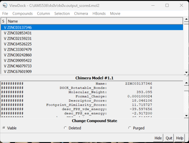
| + | Before loading the docked molecules, open a new session in Chimera and open your protein only .pdb file. Next go to Tools → Surface/Binding Analysis → ViewDock. Choose the 4s0v.output_scored.mol2 file you just transferred to your computer. A dialogue box will appear - choose the version of Dock you used to rescore the docked molecules. For this system we used Dock6, click 'OK'. Be patient, it may take a while to load. | ||
| − | + | A dialogue box will appear: | |
| + | [[File: viewDockboxs.png|center]] | ||
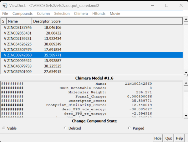
| + | Here you will see the names of all the virtually screened molecules. Clicking on each one will bring up the ligand inside the protein. You can also show different columns with information on each molecule. Click on Column → Show and all your column options will appear. Choose the one you are most interested in - for example Descriptor_Score. Your ViewDock box will now look like: | ||
| + | [[File: descriptorscorebox.png|center]] | ||
| − | + | Clicking on the name of the column sorts the molecules. By doing this, you can choose the molecules you wish to investigate further (based on descriptor score, MW, etc.) | |
Latest revision as of 16:44, 19 February 2024
Contents
- 1 Introduction
- 2 Preparation of the ligand and protein
- 3 Creating the Protein Binding Site Surface
- 4 Box and Grid Generation
- 5 Energy Minimization
- 6 DOCK
- 7 Virtual Screening of a Ligand Library
- 8 Cartesian Minimization of Virtually Screened Small Molecules
- 9 Rescoring and Ranking Virtually Screened Molecules
Introduction
This tutorial will walk you through the steps necessary for using the DOCK software package. Many drugs are small molecular compounds that attach, or bind, to a protein in our bodies to change how that protein functions. By changing the function of a protein we can treat disease and help people manage symptoms of disorders. Traditionally drug discovery was done through a type of "trial and error" process called High Throughput Screening. Scientists would chemically make, or buy, thousands of small compounds and expose them to cells. They would then observe how the cells responded, either favorably/unfavorably/no effect. This method is time consuming and expensive. It would be better if the scientific community could "virtually screen" these molecules using a computer before creating/buying them - thereby focusing the cost and effort on those which showed the most promising computational results. The DOCK software brings this drug discovery process into the 21st century and uses computers to bind these small molecular compounds to a protein and evaluate the results. DOCK uses algorithms to bring together the small molecule, known as the ligand, and the larger protein, and "DOCK" them together. Our tutorial will walk you through preparing a protein and ligand for docking using an example complex from the protein data bank (https://www.rcsb.org/), complex # 4S0V.
The following steps will be followed:
- Setting up your environment
- Downloading a protein from the PDB database
- Determining if there are any missing loops in the structure and if they need to be modeled
- Preparing the ligand
- Preparing the protein
- Finding the binding site of the protein
You will need certain skills to successfully complete this tutorial. This website has tutorials for the following:
This tutorial will be using PDB#4S0V as an example. Keep in mind that when you work on your own project to replace any reference to 4S0V with your own protein number.
Learning Objectives
- Understand why DOCK was created and its current role in drug design
- Gain the ability perform virtual screening of small molecular compounds to a protein from the Protein Data Base (https://www.rcsb.org/)
Setting Up Your Environment
Before we get started working with molecules it's a good idea to set up your directory structure on Seawulf to keep everything organized. The following directory structure should be created:
Downloading a protein from the PDB database
The first step is to download a protein complex from the PDB. As mentioned, this tutorial will be using #4S0V throughout. On the right side of the top banner you will see a search bar:
.Simply type in 4S0V and press enter. The resulting protein complex will be displayed.
On the right hand side, click on Download Files, then choose PDB Format.
That's it! The pdb file is now saved to your local computer.
Preparation of the ligand and protein
The following steps will show you how to prepare the protein and ligand structures to be used with DOCK. All steps in this section will be done using Chimera. These steps are very important - if your initial structure is not prepared properly, all downstream analysis can potentially be incorrect. This section will show you how to:
- Evaluate the structure to determine if there are any missing loops
- Prepare the protein structure
- Prepare the ligand structure
Evaluating the Structure
Open the previously downloaded .pdb file into Chimera. The first thing you want to look for are missing loops. A missing loop will be indicated by a dashed line in the structure:
The first decision you'll need to make is if these missing loops are important in your model. This decision is made by determining if the missing loop is close to the binding site. If it is far enough away, it probably won't affect the dynamics of the protein/ligand interaction and can be left alone. If the missing section is close to the binding site, you may want to fix it to more accurately model the binding site and the protein/ligand interaction.
To determine the distance between the missing loop and the binding site:
- Select an atom at near the start of the missing section (hold the ctrl button while clicking it)
- Select another atom near the binding site (hold ctrl + shift while clicking the second atom)
- Go to Tools → Structure Analysis → Distances
A dialogue box will appear:
Click the 'create' button and the distances between the two selected atoms will appear in the box. With this box open you can clear your selection (Select → Clear Selection) and then choose two more atoms. When 'Create' is again pressed, the second distance will be added to the dialogue box.
If you determine that you want to re-create the missing sections, go to Tools → Surface Editing → Model/Refine Loops. Two dialogue boxes will appear:
this box shows the sequence of amino acids in your structure.
The second box is the important one for this step. This has the required inputs you need to give Chimera so it can re-model the missing loops:
in this box choose 'non-terminal missing structure' and click 'Apply'. You can monitor the progress of Modeller in the lower left hand corner of the display. Once it has finished, another dialogue box will appear showing you the five choices of models for the missing sections.
As you click on each of the results, the re-created missing section will show up. Decide which one you want to keep, highlight it and save the file by choosing File → Save PDB. In the dialogue box, be sure to give this file a new name so as not to overwrite the original 4s0v.pdb file, something similar to 4s0v_loops_fixed.pdb. In the 'Save models' section, choose the model number you chose above. To confirm that everything has worked correctly, close your current session in Chimera and open 4s0v_loops_fixed.pdb. You should now see no dashed lines and only the structure with the re-created loops.
You are now ready to move onto preparing the ligand and protein structures for docking.
Preparing the Protein file
The first step in preparing the protein is to get the protein structure alone in a .pdb file. To do this:
- Select an atom on the protein
- Press the up arrow until the entire protein is selected
- Go to Select → Invert (all models). This will change the selection from the protein to everything else in the structure
- Go to Actions → Atoms/Bonds → Delete
- Save the structure with a new file name (i.e. 4s0v_protein_only.pdb). Your pdb file will now look similar to this:
At this point we also need to generate a .mol2 file for the structure in this state. Go to File → Save Mol2 and give the file a descriptive name such as 4s0v_protein_no_hydrogens_no_charges.mol2
There are now two more steps necessary for its preparation:
- Adding hydrogens
- Adding charge
To add hydrogen atoms click on: Tools → Structure Editing → AddH. This command will cause the following dialogue box to appear:
Click 'OK'. When the program is finished, the bottom left-hand side will say "Hydrogens added" but you won't see any change in the structure. It's good practice to make sure that the program worked properly by showing the atoms at a small area of the protein and ensuring hydrogens were added. To do with we're going to use the 'zone' command which is quite useful:
- Click on one atom anywhere on the protein
- Click on Select → Zone. This will cause the following dialogue box to appear:
make sure to click the same options as shown above and click on 'OK'. Go to Actions → Atoms/Bonds → show and the atoms in the atoms in the selected area will be shown. If the hydrogen atoms were successfully added you'll see structure similar to:
and you can see the white ends to the atoms which are the hydrogens. The final step is to add charges to the protein. Before you do this you should clear your selection by clicking on Select → Clear Selection. To add charges click on Tools → Structure Editing → Add Charge and the following dialogue box will show up:
Click on 'OK' and once the program is finished the bottom left hand corner will tell you what the total charge of the structure is. This number should be an integer. Your protein structure is now completely prepped and ready for docking. The final step is to save two files, a .pdb of the structure in this state and a .mol2 file. Simply go to File → Save PDB and choose a filename such as 4s0v_charges.pdb; then go to File → Save Mol2 and choose a filename such as 4s0v_protein_with_charges.mol2.
Preparing the Ligand File
The first step in preparing the ligand is the same as for the protein - we need to get the ligand structure alone in a .pdb file. To do this:
- Select an atom on the ligand
- Press the up arrow until the entire ligand is selected (you may have to press the up arrow many times)
- Go to Select → Invert (all models). This will change the selection from the ligand to everything else in the structure
- Go to Actions → Atom/Bonds → Delete
- Save the structure with a new file name (i.e. 4s0v_ligand_only.pdb). The image will look similar to this:
Before we start preparing the ligand for docking we need to again save a .mol2 file for the structure in this state. Go to File → Save Mol2 and give the file a descriptive name such as 4s0v_no_hydrogens_no_charges.mol2
Once we have the ligand saved as its own file we follow the same two steps we did for the protein:
- Add hydrogens
- Add charges
These steps are a bit more complicated for the ligand because Chimera may have mistakes and we need to do our best to determine where hydrogens should be, what the overall charge of the ligand is, and what changes we need to make to the results presented by Chimera. Once the hydrogens are added to the ligand your file should be similar to:
To determine if Chimera added hydrogens to the correct location we should look at the 2D structure of the ligand. This can be found on the pdb page where we downloaded the .pdb file.
clicking on the 2D image of the ligand brings up an enlarged image:
Another useful tip is to google the compound name of the ligand to try and find structures of it to compare against.
Once you have these two references, you'll want to start with the carbon atoms. We see on C29 there are 2 hydrogens but this should really be a methyl group (3 hydrogens). To fix this:
- select both hydrogens bonded to C29
- Actions → Atom/Bonds → Delete
- Select the carbon atom from which you just deleted the two hydrogens
- Tools → Structure Editing → Build Structure (the following dialogue box will appear):
- In the top drop down, change from 'Start Structure' to 'Modify Structure'
- Ensure the element says 'C' for carbon, and choose 4 bonds (since we want this carbon to have three hydrogens as opposed to the 2 hydrogens that Chimera gave it).
- Click 'Apply'
Your structure should now show a methyl group:
Next look at the oxygen atoms and do the same thing in determining if the protonation state of each is correct. For this structure it is, so we can move onto examining the nitrogen atoms. This is a bit trickier and it's not always obvious what the protonation state should be. A good way to determine this is to look at the original pdb file, with both the ligand and protein, with hydrogens added and determine if there are any interactions that don't seems right. To do this:
- Close your current session
- Open the original pdb that was downloaded
- Add hydrogens following the steps outlines above
- Look for interactions
Automatic protonation resulted in the addition of two hydrogens to one of the rings where, in the structure of the lone compound, the adjacent nitrogens form double bonds with surrounding carbons and are not bound to hydrogen atoms. Removing these two hydrogens preserves the native structure of the compound.
Looking at the ligand further we determined that the second hydrogen on the opposite nitrogen also didn't belong so that one was also removed. This is the final change we need to make to the ligand structure which now looks like this:
The final step is to add charges to the ligand. We follow the same steps as for the protein except after the dialogue box appear and we click 'OK', a second box will appear:
Here a knowledge of organic chemistry will be needed. Chimera sees that we removed two hydrogens so expects the ligand charge to be -2 but the overall charge of the ligand should be 0. Simply make this change in the drop down and click 'OK'. When the program is completed, you see the total charge calculated for the ligand in the lower left hand corner. This number should be an integer (or close to it). We are now done prep'ing the ligand for docking.
The final step is to again save two files, a .pdb and .mol2 of the structure in this state. Go to File → Save Mol2 and give the file a name such as 4s0v_ligand_hydrogens_charges.mol2 and File → Save PDB and give the file a name such as 4s0v_ligand_hydrogens_charges.pdb.
Final Steps
Before moving onto finding the binding site of the protein we need to move the four .mol2 files over to Seawulf. Do this using the following scp command:
scp *.mol2 username@login.seawulf.stonybrook.edu:'/gpfs/projects/AMS536/YOURYEAR/students/YOURGROUP/001.structure'
Creating the Protein Binding Site Surface
This section will walk you through the steps necessary to identify the binding site of the protein using a function within DOCK to place surface spheres along the protein.
Creating the Required Surface (DMS) File
In Chimera, open the 4s0v_protein_only.pdb file. Go to Actions → Surface → show. This will display the van der Waals surface of your protein. Your image should be similar to:
Once this is done the .dms file needs to be generated by clicking on Tools → Structure Editing → Write DMS. A dialogue box will appear where you need to give the file a name, such as 4s0v_surface.dms. Once this file is saved, we need to make sure that nothing was unintended happened with DOCK during its generation. We do this by overlaying the .dms file with the protein_only file. To do this, close your current session, open the 4s0v_protein_only.pdb and then open the 4s0v_surface.dms. If everything worked as it should you should see an image similar to:
As you can see, the small dots (which is the .dms file) is perfectly aligned over the protein structure. Now that we have verified that everything looks good, we can continue.
Generating Spheres for the Binding Site
Now that we have a .dms file, we need to find the binding site of the protein using a DOCK program called sphgen. This program is run on the command line on Seawulf. In order for it to run properly you need to scp the .dms file to the 002.surface_spheres directory using the command:
scp filename.dms username@login.seawulf.stonybrook.edu:'/gpfs/projects/AMS536/YOURYEAR/students/YOURGROUP/002.surface_spheres'
Once the file is in your 002.surface_spheres directory you need to create a file to run sphgen. Type:
vi INSPH
this will open a new text document with the name INSPH. Put the following in the document replacing the filenames with your specific files:
 4s0v_surface.dms
 R
 X
 0.0
 4.0
 1.4
 4s0v_binding_spheres.sph
Note that the first and last lines need to be updated to be the name of your files. Save this file and return to the command line using the command:
sphgen -i INSPH -o OUTSPH
When this is completed you will see the 4sv0_binding_spheres.sph in your directory. Once again we need to verify that this file was generated properly. Do this by comparing it to the original .pdb. Using scp, move the output file (in this case 4s0v_binding_spheres.sph) back to your local computer and open the file in a new Chimera session. In the same session, open the original .pdb file and the two structures should be aligned to each other. Your image should be similar to:
As you can see, the ribbon of the original file is aligned to the spheres we just generated. At this point we can move onto the next step of selecting the spheres within the binding site of the protein.
Binding Site Spheres
This step runs a DOCK program called sphere_selector which is again run on the command line. Log back in to Seawulf and move to your 002.surface_spheres directory. Then type:
sphere_selector 4s0v_binding_spheres.sph ../001.structure/4s0v_ligand_hydrogens_charges.mol2 10.0
When this program has successfully completed you'll see a new file in your directory called selected_spheres.sph. This file generated spheres which should line up with the binding site of the protein. We need to verify this in Chimera:
- scp selected_spheres.sph to your local computer
- Close any open sessions you have in Chimera
- In Chimera open selected_spheres.sph
- In the current session, open the original protein/ligand complex (4s0v.pdb)
- You should see the spheres located within the binding site of the protein, similar to:
While this looks good we should verify that the spheres are actually where the ligand is. Let's do this by selecting the spheres, hiding them from view, and verifying the ligand is in the same location:
- Hold down ctrl and click on a sphere
- Press the up arrow until all spheres are selected
- Actions → Atoms/Bonds → hide
- Verify the ligand is where the spheres were
and we see the ligand is where the spheres were so we can be confident in our work so far.
Box and Grid Generation
The next step in the docking process is to generate energy interactions between the atoms of the protein and ligand. If this was done for the whole complex it would take too long to run to be useful. To get around this computationally expensive step, dock uses a box/grid method. We will define a box around the area of interest for the protein/ligand and DOCK will generate a grid within this box which will be used in the energy calculations.
Generating the Box
To generate the box we will be working again on the command line using a DOCK program called showbox. Start by logging into Seawulf and navigating to your 003.gridbox directory. We need to make a new file called showbox.in by typing:
vi showbox.in
This will create a new file, with a filename of showbox.in and open it in vi. The following commands need to be typed:
     Y
     8.0
     ../002.surface_spheres/selected_spheres.sph
     1
     4s0v.box.pdb
Remember to change the last line to be a filename with the number of protein you are working with. The second line of this code (8.0) is telling dock how many angstroms from the selected spheres to draw the box. Depending on your system you may need to modify this number.
To run this file, simply type:
showbox < showbox.in
If showbox was successful the file 4s0v.box.pdb will now be in your directory.
Generating the Grid
Now that we have our box defined we need to instruct DOCK to generate the grid within it. We do this using a DOCK program called grid:
vi grid.in
This command will generate and open a file named grid.in. The commands to be typed into this file are:
   allow_non_integral_charges                no
   compute_grids                             yes
   grid_spacing                              0.4
   output_molecule                           no
   contact_score                             no
   energy_score                              yes
   energy_cutoff_distance                    9999
   atom_model                                a
   attractive_exponent                       6
   repulsive_exponent                        9
   distance_dielectric                       yes
   dielectric_factor                         4.
   bump_filter                               yes
   bump_overlap                              0.75
   receptor_file                              ../001.structure/4s0v_protein_hydrogens_charges.mol2
   box_file                                  4s0v.box.pdb
   vdw_definition_file                       /gpfs/projects/AMS536/zzz.programs/dock6.9_release/parameters/vdw_AMBER_parm99.defn
   score_grid_prefix                         grid
The only change you need to make to the above commands is the receptor_file and box_file to reflect the files you previously generated.
Once this file is saved, run it:
grid -i grid.in -o 4s0vGridInfo.out
Be patient, this step might take a few minutes to run. You will know it's worked successfully if you see:
- grid.bmp
- grid.nrg
- 4s0vGridInfo.out
in your directory. With the box and grid successfully generated we are ready to move onto the energy minimization step.
Energy Minimization
At its core, DOCK is finding interactions between a protein and ligand by looking at energy interactions between atoms. In order for DOCK to give the most accurate results we need to ensure that the ligand is at its lowest energy state before docking it into the binding site of the protein.
Ligand Minimization
For this section we will be working in the 004.energy_min directory and will be using the dock6 command. Again we need to generate the input file that dock6 needs:
vi min.in
Once in vi the following lines need to be typed in:
  conformer_search_type                                        rigid
  use_internal_energy                                          yes
  internal_energy_rep_exp                                      12
  internal_energy_cutoff                                       100.0
  ligand_atom_file                                             ../001.structure/4s0v_ligand_hydrogens_charges.mol2
  limit_max_ligands                                            no
  skip_molecule                                                no
  read_mol_solvation                                           no
  calculate_rmsd                                               yes
  use_rmsd_reference_mol                                       yes
  rmsd_reference_filename                                      ../001.structure/4s0v_ligand_hydrogens_charges.mol2
  use_database_filter                                          no
  orient_ligand                                                no
  bump_filter                                                  no
  score_molecules                                              yes
  contact_score_primary                                        no
  contact_score_secondary                                      no
  grid_score_primary                                           yes
  grid_score_secondary                                         no
  grid_score_rep_rad_scale                                     1
  grid_score_vdw_scale                                         1
  grid_score_es_scale                                          1
  grid_score_grid_prefix                                       ../003.gridbox/grid
  multigrid_score_secondary                                    no
  dock3.5_score_secondary                                      no
  continuous_score_secondary                                   no
  footprint_similarity_score_secondary                         no
  pharmacophore_score_secondary                                no
  descriptor_score_secondary                                   no
  gbsa_zou_score_secondary                                     no
  gbsa_hawkins_score_secondary                                 no
  SASA_score_secondary                                         no
  amber_score_secondary                                        no
  minimize_ligand                                              yes
  simplex_max_iterations                                       1000
  simplex_tors_premin_iterations                               0
  simplex_max_cycles                                           1
  simplex_score_converge                                       0.1
  simplex_cycle_converge                                       1.0
  simplex_trans_step                                           1.0
  simplex_rot_step                                             0.1
  simplex_tors_step                                            10.0
  simplex_random_seed                                          0
  simplex_restraint_min                                        yes
  simplex_coefficient_restraint                                10.0
  atom_model                                                   all
  vdw_defn_file                                                /gpfs/projects/AMS536/zzz.programs/dock6.9_release/parameters/vdw_AMBER_parm99.defn
  flex_defn_file                                               /gpfs/projects/AMS536/zzz.programs/dock6.9_release/parameters/flex.defn
  flex_drive_file                                              /gpfs/projects/AMS536/zzz.programs/dock6.9_release/parameters/flex_drive.tbl
  ligand_outfile_prefix                                        4s0v.lig.min
  write_orientations                                           no
  num_scored_conformers                                        1
  rank_ligands                                                 no
And the file is run with the following command:
dock6 -i min.in -o min.out
After successful completion of the program two new files will be in your directory:
- min.out
- 4s0v.lig.min.mol2
scp the .mol2 file back to your local computer. To view the changes that dock made to the structure, and open the 4s0v.lig.min.mol2 file in Chimera and in the same session, open the 4s0v_ligand_with_chareg.pdb file. Remember the 4s0v_ligand_with_charge.pdb is the file we saved after making the protonation changes to the ligand. You should see something similar to:
And you can see DOCK has made small changes to the ligand structure.
Footprint Analysis
At its core, DOCK can be thought of as a program which evaluates, minimizes, and uses the electrostatic and VDW interactions between the ligand and protein to determine how they bind to each other. A footprint analysis is a way to visualize these interactions and possibly be used to design new ligands with the same, or better, set of energetics. The steps in this section will be done on Seawulf in the 005.footprint directory. We will be using the dock6 command and again need to create an input file:
vi footprint.in
The following lines needed to be typed into the newly created file:
  conformer_search_type                                        rigid
  use_internal_energy                                          no
  ligand_atom_file                                             ../004.energy_min/4s0v.lig.min_scored.mol2
  limit_max_ligands                                            no
  skip_molecule                                                no
  read_mol_solvation                                           no
  calculate_rmsd                                               no
  use_database_filter                                          no
  orient_ligand                                                no
  bump_filter                                                  no
  score_molecules                                              yes
  contact_score_primary                                        no
  contact_score_secondary                                      no
  grid_score_primary                                           no
  grid_score_secondary                                         no
  multigrid_score_primary                                      no
  multigrid_score_secondary                                    no
  dock3.5_score_primary                                        no
  dock3.5_score_secondary                                      no
  continuous_score_primary                                     no
  continuous_score_secondary                                   no
  footprint_similarity_score_primary                           yes
  footprint_similarity_score_secondary                         no
  fps_score_use_footprint_reference_mol2                       yes
  fps_score_footprint_reference_mol2_filename                  ../001.structure/4s0v_ligand_hydrogens_charges.mol2
  fps_score_foot_compare_type                                  Euclidean
  fps_score_normalize_foot                                     no
  fps_score_foot_comp_all_residue                              yes
  fps_score_receptor_filename                                  ../001.structure/4s0v_protein_hydrogens_charges.mol2
  fps_score_vdw_att_exp                                        6
  fps_score_vdw_rep_exp                                        9
  fps_score_vdw_rep_rad_scale                                  1
  fps_score_use_distance_dependent_dielectric                  yes
  fps_score_dielectric                                         4.0
  fps_score_vdw_fp_scale                                       1
  fps_score_es_fp_scale                                        1
  fps_score_hb_fp_scale                                        0
  pharmacophore_score_secondary                                no
  descriptor_score_secondary                                   no
  gbsa_zou_score_secondary                                     no
  gbsa_hawkins_score_secondary                                 no
  SASA_score_secondary                                         no
  amber_score_secondary                                        no
  minimize_ligand                                              no
  atom_model                                                   all
  vdw_defn_file                                                /gpfs/projects/AMS536/zzz.programs/dock6.9_release/parameters/vdw_AMBER_parm99.defn
  flex_defn_file                                               /gpfs/projects/AMS536/zzz.programs/dock6.9_release/parameters/flex.defn
  flex_drive_file                                              /gpfs/projects/AMS536/zzz.programs/dock6.9_release/parameters/flex_drive.tbl
  ligand_outfile_prefix                                        4s0v_footprint.out
  write_footprints                                             yes
  write_hbonds                                                 yes
  write_orientations                                           no
  num_scored_conformers                                        1
  rank_ligands                                                 no
to generate the footprint of the ligand/protein interaction type:
dock6 -i footprint.in
Again, you will know the program successfully ran if the following three files are now in your directory:
- 4s0v_footprint.out_footprint_scored.txt
- 4s0v_footprint.out_hbond_scored.txt
- 4s0v_footprint.out_scored.mol2
In order to view/analyze these results we need to use a python script that is located in the class directory. Copy it over to your 005.footprint directory with the following command:
cp /gpfs/projects/AMS536/2020/536_class/steve_ta/footprint_test_1.21.2020/plot_footprint_single_magnitude.py .
To run this script type:
python plot_footprint_single_magnitude.py 4s0v_footprint.out_footprint_scored.txt 50
If you get an error when running this script you may need to load a module in order to access python. Try typing:
module load anaconda/2
and then re-running the python script. It should work now.
Once the script is completed you will see a .pdf file in your directory. scp this file back to your local computer. The file contains two plots that shows the energetic signature for the 50 most significant residues and will look similar to:
DOCK
We will be exploring three different options of the DOCK program:
- Rigid Docking
- Fixed Anchor Docking
- Flexible Docking
Each option has it's own pros and cons and your individual system should dictate which option you choose. Note: In the input file for each of these options has a line:
num_scored_conformers 1
Changing this number will change the number of conformations saved from the docking session.
Rigid Docking
When using rigid docking, the DOCK program does not sample different conformations of the ligand to try and find the most energetically stable. It simply treats the ligand as a rigid structure and tries to fit it into the binding site of the protein. For this step we will be using the energy minimized ligand file we generated above. This section will again be completed on Seawulf, please move to the 006.rigid_docking directory.
Again we need an input file that can be created using the command:
vi rigid.in
The following lines need to be typed into the file:
 conformer_search_type                                        rigid
 write_fragment_libraries                                     no
 user_specified_anchor                                        no
 limit_max_anchors                                            no
 min_anchor_size                                              5
 pruning_use_clustering                                       yes
 pruning_max_orients                                          1000
 pruning_clustering_cutoff                                    100
 pruning_conformer_score_cutoff                               100.0
 pruning_conformer_score_scaling_factor                       1.0
 use_clash_overlap                                            no
 write_growth_tree                                            no
 use_internal_energy                                          yes
 internal_energy_rep_exp                                      12
 internal_energy_cutoff                                       100.0
 ligand_atom_file                                             ../004.energy_min/4s0v.lig.min_scored.mol2
 limit_max_ligands                                            no
 skip_molecule                                                no
 read_mol_solvation                                           no
 calculate_rmsd                                               yes
 use_rmsd_reference_mol                                       yes
 rmsd_reference_filename                                      ../004.energy_min/4s0v.lig.min_scored.mol2
 use_database_filter                                          no
 orient_ligand                                                yes
 automated_matching                                           yes
 receptor_site_file                                           ../002.surface_spheres/selected_spheres.sph
 max_orientations                                             1000
 critical_points                                              no
 chemical_matching                                            no
 use_ligand_spheres                                           no
 bump_filter                                                  no
 score_molecules                                              yes
 contact_score_primary                                        no
 contact_score_secondary                                      no
 grid_score_primary                                           yes
 grid_score_secondary                                         no
 grid_score_rep_rad_scale                                     1
 grid_score_vdw_scale                                         1
 grid_score_es_scale                                          1
 grid_score_grid_prefix                                       ../003.gridbox/grid
 multigrid_score_secondary                                    no
 dock3.5_score_secondary                                      no
 continuous_score_secondary                                   no
 footprint_similarity_score_secondary                         no
 pharmacophore_score_secondary                                no
 descriptor_score_secondary                                   no
 gbsa_zou_score_secondary                                     no
 gbsa_hawkins_score_secondary                                 no
 SASA_score_secondary                                         no
 amber_score_secondary                                        no
 minimize_ligand                                              yes
 minimize_anchor                                              yes
 minimize_flexible_growth                                     yes
 use_advanced_simplex_parameters                              no
 simplex_max_cycles                                           1
 simplex_score_converge                                       0.1
 simplex_cycle_converge                                       1.0
 simplex_trans_step                                           1.0
 simplex_rot_step                                             0.1
 simplex_tors_step                                            10.0
 simplex_anchor_max_iterations                                500
 simplex_grow_max_iterations                                  500
 simplex_grow_tors_premin_iterations                          0
 simplex_random_seed                                          0
 simplex_restraint_min                                        no
 atom_model                                                   all
 vdw_defn_file                                                /gpfs/projects/AMS536/zzz.programs/dock6.9_release/parameters/vdw_AMBER_parm99.defn
 flex_defn_file                                               /gpfs/projects/AMS536/zzz.programs/dock6.9_release/parameters/flex.defn
 flex_drive_file                                              /gpfs/projects/AMS536/zzz.programs/dock6.9_release/parameters/flex_drive.tbl
 ligand_outfile_prefix                                        rigid.out
 write_orientations                                           no
 num_scored_conformers                                        1
 rank_ligands                                                 no
Remember to again change the necessary lines to point to your specific files. Once this is completed run the program by typing:
dock6 -i rigid.in -o rigid.out
Again, be patient as this may take a few minutes to complete. Once it's done running you will see two new files in your directory:
- rigid.out_scored.mol2
- rigid.out
scp the .mol2 file over to your local computer. Start a new session in Chimera and open the energy minimized ligand file from the previous step and the rigid docked ligand you just created (4s0v.lig.min_scored.mol2 and rigid.out_scored.mol2) to view the differences between the energy minimized ligand and DOCK's attempt to rigid dock that structure into the protein.
Looking at this file we see that the two are very similar to each other.
Now we can look at the other file that dock generated, rigid.out. If we scroll to the bottom you will see grid scoring for this run:
Fixed Anchor Docking
The next DOCK option we will be looking at is called 'Fixed Anchor Docking'. For this option, DOCK cuts the ligand into fragments along its rotatable bonds. It then chooses the largest fragment as the 'anchor' and orients this fragment into the binding site of the protein. Once this is completed, the next fragments are added to the ligand, orientating them such that their energy is minimized but keeping them as rigid bodies. Comparing this to Rigid Docking, we see that more conformational sampling is being done but still within limits since each fragment is considered rigid.
We'll be working on the command line again, please move to the 007.fixed_anchor_docking directory and create an input file called fixed.in:
vi fixed.in
and type the following lines:
 conformer_search_type                                        flex
 write_fragment_libraries                                     no
 user_specified_anchor                                        no
 limit_max_anchors                                            no
 min_anchor_size                                              5
 pruning_use_clustering                                       yes
 pruning_max_orients                                          1000
 pruning_clustering_cutoff                                    100
 pruning_conformer_score_cutoff                               100.0
 pruning_conformer_score_scaling_factor                       1.0
 use_clash_overlap                                            no
 write_growth_tree                                            no
 use_internal_energy                                          yes
 internal_energy_rep_exp                                      12
 internal_energy_cutoff                                       100.0
 ligand_atom_file                                             ../004.energy_min/4s0v.lig.min_scored.mol2
 limit_max_ligands                                            no
 skip_molecule                                                no
 read_mol_solvation                                           no
 calculate_rmsd                                               yes
 use_rmsd_reference_mol                                       yes
 rmsd_reference_filename                                      ../004.energy_min/4s0v.lig.min_scored.mol2
 use_database_filter                                          no
 orient_ligand                                                no
 bump_filter                                                  no
 score_molecules                                              yes
 contact_score_primary                                        no
 contact_score_secondary                                      no
 grid_score_primary                                           yes
 grid_score_secondary                                         no
 grid_score_rep_rad_scale                                     1
 grid_score_vdw_scale                                         1
 grid_score_es_scale                                          1
 grid_score_grid_prefix                                       ../003.gridbox/grid
 multigrid_score_secondary                                    no
 dock3.5_score_secondary                                      no
 continuous_score_secondary                                   no
 footprint_similarity_score_secondary                         no
 pharmacophore_score_secondary                                no
 descriptor_score_secondary                                   no
 gbsa_zou_score_secondary                                     no
 gbsa_hawkins_score_secondary                                 no
 SASA_score_secondary                                         no
 amber_score_secondary                                        no
 minimize_ligand                                              yes
 minimize_anchor                                              yes
 minimize_flexible_growth                                     yes
 use_advanced_simplex_parameters                              no
 simplex_max_cycles                                           1
 simplex_score_converge                                       0.1
 simplex_cycle_converge                                       1
 simplex_trans_step                                           1
 simplex_rot_step                                             0.1
 simplex_tors_step                                            10.0
 simplex_anchor_max_iterations                                500
 simplex_grow_max_iterations                                  500
 simplex_grow_tors_premin_iterations                          0
 simplex_random_seed                                          0
 simplex_restraint_min                                        no
 atom_model                                                   all
 vdw_defn_file                                                /gpfs/projects/AMS536/zzz.programs/dock6.9_release/parameters/vdw_AMBER_parm99.defn
 flex_defn_file                                               /gpfs/projects/AMS536/zzz.programs/dock6.9_release/parameters/flex.defn
 flex_drive_file                                              /gpfs/projects/AMS536/zzz.programs/dock6.9_release/parameters/flex_drive.tbl
 ligand_outfile_prefix                                        4s0v_fixed_output
 write_orientations                                           no
 num_scored_conformers                                        1
 rank_ligands                                                 no
Again, change the necessary lines to point to your specific files. To run this file type:
dock6 -i fixed.in -o fixed.out
Once it's done running you will see two new files in your directory:
- fixed.out
- 4s0v_fixed_output_scored.mol2
scp the .mol2 file over to your local computer. Start a new session in Chimera and open the energy minimized ligand file from the previous step and the fixed anchor docked ligand you just created (4s0v.lig.min_scored.mol2 and 4s0v_fixed_output_scored.mol2) to view the differences between the energy minimized ligand and DOCK's attempt to place that structure using its fixed anchor algorithm. Your image should be similar to:
And looking at the grid score in fixed.out we see:
Let's now open both .mol2 files in Chimera and see how they compare to each other:
Doing this allows us to see the differences in the poses of the two different docking methods.
Flexible Docking
The final docking method we're going to look at is called flexible docking. This is the most computationally expensive of the three methods, because now DOCK will sample all conformations of all rotatable bonds within the ligand attempting to minimize the energetics of the ligand. Once again we will be working on the command line in Seawulf, but now in your 008.flex_docking directory.
Create your input file:
vi flex.in
And type the following lines into your input file:
 conformer_search_type                                        flex
 write_fragment_libraries                                     no
 user_specified_anchor                                        no
 limit_max_anchors                                            no
 min_anchor_size                                              5
 pruning_use_clustering                                       yes
 pruning_max_orients                                          1000
 pruning_clustering_cutoff                                    100
 pruning_conformer_score_cutoff                               100.0
 pruning_conformer_score_scaling_factor                       1.0
 use_clash_overlap                                            no
 write_growth_tree                                            no
 use_internal_energy                                          yes
 internal_energy_rep_exp                                      12
 internal_energy_cutoff                                       100.0
 ligand_atom_file                                             ../004.energy_min/4s0v.lig.min_scored.mol2
 limit_max_ligands                                            no
 skip_molecule                                                no
 read_mol_solvation                                           no
 calculate_rmsd                                               yes
 use_rmsd_reference_mol                                       yes
 rmsd_reference_filename                                      ../004.energy_min/4s0v.lig.min_scored.mol2
 use_database_filter                                          no
 orient_ligand                                                yes
 automated_matching                                           yes
 receptor_site_file                                           ../002.surface_spheres/selected_spheres.sph
 max_orientations                                             1000
 critical_points                                              no
 chemical_matching                                            no
 use_ligand_spheres                                           no
 bump_filter                                                  no
 score_molecules                                              yes
 contact_score_primary                                        no
 contact_score_secondary                                      no
 grid_score_primary                                           yes
 grid_score_secondary                                         no
 grid_score_rep_rad_scale                                     1
 grid_score_vdw_scale                                         1
 grid_score_es_scale                                          1
 grid_score_grid_prefix                                       ../003.gridbox/grid
 multigrid_score_secondary                                    no
 dock3.5_score_secondary                                      no
 continuous_score_secondary                                   no
 footprint_similarity_score_secondary                         no
 pharmacophore_score_secondary                                no
 descriptor_score_secondary                                   no
 gbsa_zou_score_secondary                                     no
 gbsa_hawkins_score_secondary                                 no
 SASA_score_secondary                                         no
 amber_score_secondary                                        no
 minimize_ligand                                              yes
 minimize_anchor                                              yes
 minimize_flexible_growth                                     yes
 use_advanced_simplex_parameters                              no
 simplex_max_cycles                                           1
 simplex_score_converge                                       0.1
 simplex_cycle_converge                                       1.0
 simplex_trans_step                                           1.0
 simplex_rot_step                                             0.1
 simplex_tors_step                                            10.0
 simplex_anchor_max_iterations                                500
 simplex_grow_max_iterations                                  500
 simplex_grow_tors_premin_iterations                          0
 simplex_random_seed                                          0
 simplex_restraint_min                                        no
 atom_model                                                   all
 vdw_defn_file                                                /gpfs/projects/AMS536/zzz.programs/dock6.9_release/parameters/vdw_AMBER_parm99.defn
 flex_defn_file                                               /gpfs/projects/AMS536/zzz.programs/dock6.9_release/parameters/flex.defn
 flex_drive_file                                              /gpfs/projects/AMS536/zzz.programs/dock6.9_release/parameters/flex_drive.tbl
 ligand_outfile_prefix                                        flex.out
 write_orientations                                           no
 num_scored_conformers                                        1
 rank_ligands                                                 no
and run the file using the command:
dock6 -i flex.in -o flex.out
When the program has finished running you will see two new files in your directory:
- flex.out
- flex.out_scored.mol2
again, scp the .mol2 file to your local computer and open it into a new session in Chimera. Overlaying this file with the energy minimized ligand we see:
Looking at the grid scores from flex.out:
Its interesting to now load the results from all three docking methods, along with the energy minimized ligand, and see the differences:
In this image:
- tan is rigid docking
- green is the energy minimized ligand
- blue is the flexible docking
- pink is the fixed anchor docking
Virtual Screening of a Ligand Library
Up to this point we have been docking one molecule, the ligand that was in the protein/ligand complex from the pdb. But DOCK has the ability to find interactions between the protein and many different small molecules, finding the top binding ligands. This allows us to "screen" thousands of molecules but only spend time digging into the details of the top results. For this tutorial, we have created a file, VS_library_5K.mol2, which contains all the information needed on the molecules we wish to screen. Again we will be working on the command line in the 009.virtual_screening directory.
Let's create our input file:
vi virtual.in
which needs to have the following lines typed in:
    conformer_search_type                                        flex
    write_fragment_libraries                                     no
    user_specified_anchor                                        no
    limit_max_anchors                                            no
    min_anchor_size                                              5
    pruning_use_clustering                                       yes
    pruning_max_orients                                          1000
    pruning_clustering_cutoff                                    100
    pruning_conformer_score_cutoff                               100.0
    pruning_conformer_score_scaling_factor                       1.0
    use_clash_overlap                                            no
    write_growth_tree                                            no
    use_internal_energy                                          yes
    internal_energy_rep_exp                                      9
    internal_energy_cutoff                                       100.0
    ligand_atom_file                                             /gpfs/projects/AMS536/zzz.programs/VS_library_5K.mol2
    limit_max_ligands                                            no
    skip_molecule                                                no
    read_mol_solvation                                           no
    calculate_rmsd                                               no
    use_database_filter                                          no
    orient_ligand                                                yes
    automated_matching                                           yes
    receptor_site_file                                           ../002.surface_spheres/selected_spheres.sph
    max_orientations                                             1000
    critical_points                                              no
    chemical_matching                                            no
    use_ligand_spheres                                           no
    bump_filter                                                  no
    score_molecules                                              yes
    contact_score_primary                                        no
    contact_score_secondary                                      no
    grid_score_primary                                           yes
    grid_score_secondary                                         no
    grid_score_rep_rad_scale                                     1
    grid_score_vdw_scale                                         1
    grid_score_es_scale                                          1
    grid_score_grid_prefix                                       ../003.gridbox/grid
    multigrid_score_secondary                                    no
    dock3.5_score_secondary                                      no
    continuous_score_secondary                                   no
    footprint_similarity_score_secondary                         no
    pharmacophore_score_secondary                                no
    descriptor_score_secondary                                   no
    gbsa_zou_score_secondary                                     no
    gbsa_hawkins_score_secondary                                 no
    SASA_score_secondary                                         no
    amber_score_secondary                                        no
    minimize_ligand                                              yes
    minimize_anchor                                              yes
    minimize_flexible_growth                                     yes
    use_advanced_simplex_parameters                              no
    simplex_max_cycles                                           1
    simplex_score_converge                                       0.1
    simplex_cycle_converge                                       1.0
    simplex_trans_step                                           1.0
    simplex_rot_step                                             0.1
    simplex_tors_step                                            10.0
    simplex_anchor_max_iterations                                500
    simplex_grow_max_iterations                                  500
    simplex_grow_tors_premin_iterations                          0
    simplex_random_seed                                          0
    simplex_restraint_min                                        no
    atom_model                                                   all
    vdw_defn_file                                                /gpfs/projects/AMS536/zzz.programs/dock6.9_release/parameters/vdw_AMBER_parm99.defn
    flex_defn_file                                               /gpfs/projects/AMS536/zzz.programs/dock6.9_release/parameters/flex.defn
    flex_drive_file                                              /gpfs/projects/AMS536/zzz.programs/dock6.9_release/parameters/flex_drive.tbl
    ligand_outfile_prefix                                        virtual.out
    write_orientations                                           no
    num_scored_conformers                                        1
    rank_ligands                                                 no
Running DOCK on 5000 molecules CANNOT be done on the login node of Seawulf. You will crash the system and have your login information suspended. All computationally intensive jobs such as this need to be submitted to Seawulf using the scheduler, Slurm. To do this you need to create a slurm script, which is just a text file that tells Seawulf what you want to run.
Create your slurm script
vi 4s0v_virtual.slurm
The contents of the slurm script are:
  #!/bin/bash
  #
  #SBATCH --job-name=4s0v_vs_tutorial
  #SBATCH --output=vs_output.txt
  #SBATCH --ntasks=24
  #SBATCH --nodes=6
  #SBATCH --time=48:00:00
  #SBATCH -p long-24core

  module load intel/mpi/64/2018/18.0.3

  mpirun -np 144 dock6.mpi -i virtual.in -o virtual.out
To get this script to run, on the command line, type:
 module load slurm
 sbatch 4s0v_virtual.slurm
This script is virtually screening 5,000 molecules and could take up to 48 hours to complete. After 48 hours, slurm will stop the job even if all 5,000 compounds haven't been docked yet. At any point while it's running, if you want to see how many molecules have been docked so far, simply type:
grep Molecule: virtual.out | wc -l
be sure to type the above command from your 009.virtual_screening directory.
After 48 hours, our script stopped running and 4549 molecules had been docked to our protein. In order to find the top "hits" of small molecules we need to minimize the outputs which is outlined in the next section.
Cartesian Minimization of Virtually Screened Small Molecules
In order to minimize the 4549 molecules that were docked we need to create an input file. cd over to your 010.cartesian_minimization directory and create the input file:
vi min.in
and type in the following lines:
 conformer_search_type                                        rigid
 use_internal_energy                                          yes
 internal_energy_rep_exp                                      12
 internal_energy_cutoff                                       100
 ligand_atom_file                                             ../009.virtual_screening/virtual.out_scored.mol2
 limit_max_ligands                                            no
 skip_molecule                                                no
 read_mol_solvation                                           no
 calculate_rmsd                                               no
 use_database_filter                                          no
 orient_ligand                                                no
 bump_filter                                                  no
 score_molecules                                              yes
 contact_score_primary                                        no
 contact_score_secondary                                      no
 grid_score_primary                                           no
 grid_score_secondary                                         no
 multigrid_score_primary                                      no
 multigrid_score_secondary                                    no
 dock3.5_score_primary                                        no
 dock3.5_score_secondary                                      no
 continuous_score_primary                                     yes
 continuous_score_secondary                                   no
 cont_score_rec_filename                                      ../001.structure/4s0v_protein_hydrogens_charges.mol2
 cont_score_att_exp                                           6
 cont_score_rep_exp                                           12
 cont_score_rep_rad_scale                                     1
 cont_score_use_dist_dep_dielectric                           yes
 cont_score_dielectric                                        4.0
 cont_score_vdw_scale                                         1.0
 cont_score_es_scale                                          1.0
 footprint_similarity_score_secondary                         no
 pharmacophore_score_secondary                                no
 descriptor_score_secondary                                   no
 gbsa_zou_score_secondary                                     no
 gbsa_hawkins_score_secondary                                 no
 SASA_score_secondary                                         no
 amber_score_secondary                                        no
 minimize_ligand                                              yes
 simplex_max_iterations                                       1000
 simplex_tors_premin_iterations                               0
 simplex_max_cycles                                           1.0
 simplex_score_converge                                       0.1
 simplex_cycle_converge                                       1.0
 simplex_trans_step                                           1.0
 simplex_rot_step                                             0.1
 simplex_tors_step                                            10.0
 simplex_random_seed                                          0
 simplex_restraint_min                                        no
 atom_model                                                   all
 vdw_defn_file                                                /gpfs/projects/AMS536/zzz.programs/dock6.9_release/parameters/vdw_AMBER_parm99.defn
 flex_defn_file                                               /gpfs/projects/AMS536/zzz.programs/dock6.9_release/parameters/flex.defn
 flex_drive_file                                              /gpfs/projects/AMS536/zzz.programs/dock6.9_release/parameters/flex_drive.tbl
 ligand_outfile_prefix                                        4s0v.virtual_screen.min
 write_orientations                                           no
 num_scored_conformers                                        1
 rank_ligands                                                 no
Once again do NOT run this input file on the login node. You need a slurm script again:
 #!/bin/bash
 #
 #SBATCH --job-name=4s0v_minimization_tutorial
 #SBATCH --output=min_output.txt
 #SBATCH --ntasks-per-node=24
 #SBATCH --nodes=6
 #SBATCH --time=48:00:00
 #SBATCH -p long-24core

 dock6 -i min.in -o min.out
The next step to perform on the almost 5,000 molecules that were docked is to re-score them and rank them to find potential hits that can be investigated further. The next, and final section of this tutorial, will walk you through that step.
Rescoring and Ranking Virtually Screened Molecules
Once again we will be working on the command line in Seawulf and submitting our input file using a slurm script. cd to your 011.reScore directory and type:
vi rescore.in
The following lines need to be typed into rescore.in
conformer_search_type                                        rigid
use_internal_energy                                          yes
internal_energy_rep_exp                                      12
internal_energy_cutoff                                       100
ligand_atom_file                                             ../009.virtual_screening/virtual.out_scored.mol2
limit_max_ligands                                            no
skip_molecule                                                no
read_mol_solvation                                           no
calculate_rmsd                                               no
use_database_filter                                          no
orient_ligand                                                no
bump_filter                                                  no
score_molecules                                              yes
contact_score_primary                                        no
contact_score_secondary                                      no
grid_score_primary                                           no
grid_score_secondary                                         no
multigrid_score_primary                                      no
multigrid_score_secondary                                    no
dock3.5_score_primary                                        no
dock3.5_score_secondary                                      no
continuous_score_primary                                     no
continuous_score_secondary                                   no
footprint_similarity_score_primary                           no
footprint_similarity_score_secondary                         no
pharmacophore_score_primary                                  no
pharmacophore_score_secondary                                no
descriptor_score_primary                                     yes
descriptor_score_secondary                                   no
descriptor_use_grid_score                                    no
descriptor_use_multigrid_score                               no
descriptor_use_continuous_score                              no
descriptor_use_footprint_similarity                          yes
descriptor_use_pharmacophore_score                           yes
descriptor_use_hungarian                                     yes
descriptor_use_volume_overlap                                yes
descriptor_fps_score_use_footprint_reference_mol2            yes
descriptor_fps_score_footprint_reference_mol2_filename       ../004.energy_min/4s0v.lig.min_scored.mol2
descriptor_fps_score_foot_compare_type                       Euclidean
descriptor_fps_score_normalize_foot                          no
descriptor_fps_score_foot_comp_all_residue                   yes
descriptor_fps_score_receptor_filename                       ../001.structure/4s0v_protein_hydrogens_charges.mol2
descriptor_fps_score_vdw_att_exp                             6
descriptor_fps_score_vdw_rep_exp                             12
descriptor_fps_score_vdw_rep_rad_scale                       1
descriptor_fps_score_use_distance_dependent_dielectric       yes
descriptor_fps_score_dielectric                              4.0
descriptor_fps_score_vdw_fp_scale                            1
descriptor_fps_score_es_fp_scale                             1
descriptor_fps_score_hb_fp_scale                             0
descriptor_fms_score_use_ref_mol2                            yes
descriptor_fms_score_ref_mol2_filename                       ../004.energy_min/4s0v.lig.min_scored.mol2
descriptor_fms_score_write_reference_pharmacophore_mol2      no
descriptor_fms_score_write_reference_pharmacophore_txt       no
descriptor_fms_score_write_candidate_pharmacophore           no
descriptor_fms_score_write_matched_pharmacophore             no
descriptor_fms_score_compare_type                            overlap
descriptor_fms_score_full_match                              yes
descriptor_fms_score_match_rate_weight                       5.0
descriptor_fms_score_match_dist_cutoff                       1.0
descriptor_fms_score_match_proj_cutoff                       .7071
descriptor_fms_score_max_score                               20
descriptor_fingerprint_ref_filename                          ../004.energy_min/4s0v.lig.min_scored.mol2
descriptor_hms_score_ref_filename                            ../004.energy_min/4s0v.lig.min_scored.mol2
descriptor_hms_score_matching_coeff                          -5
descriptor_hms_score_rmsd_coeff                              1
descriptor_volume_score_reference_mol2_filename              ../004.energy_min/4s0v.lig.min_scored.mol2
descriptor_volume_score_overlap_compute_method               analytical
descriptor_weight_fps_score                                  1
descriptor_weight_pharmacophore_score                        1
descriptor_weight_fingerprint_tanimoto                       -1
descriptor_weight_hms_score                                  1
descriptor_weight_volume_overlap_score                       -1
gbsa_zou_score_secondary                                     no
gbsa_hawkins_score_secondary                                 no
SASA_score_secondary                                         no
amber_score_secondary                                        no
minimize_ligand                                              no
atom_model                                                   all
vdw_defn_file                                                /gpfs/projects/AMS536/zzz.programs/dock6.9_release/parameters/vdw_AMBER_parm99.defn
flex_defn_file                                               /gpfs/projects/AMS536/zzz.programs/dock6.9_release/parameters/flex.defn
flex_drive_file                                              /gpfs/projects/AMS536/zzz.programs/dock6.9_release/parameters/flex_drive.tbl
chem_defn_file                                               /gpfs/projects/AMS536/zzz.programs/dock6.9_release/parameters/chem.defn
pharmacophore_defn_file                                      /gpfs/projects/AMS536/zzz.programs/dock6.9_release/parameters/ph4.defn
ligand_outfile_prefix                                        4s0v.output
write_footprints                                             yes
write_hbonds                                                 yes
write_orientations                                           no
num_scored_conformers                                        1
rank_ligands                                                 no
and the required slurm script is:
#!/bin/bash
#
#SBATCH --job-name=4s0v_rescoring
#SBATCH --output=rescoring.txt
#SBATCH --ntasks-per-node=24
#SBATCH --nodes=6
#SBATCH --time=48:00:00
#SBATCH -p long-24core

module load intel/mpi/64/2018/18.0.3

mpirun -np 6 dock6.mpi -i rescore.in -o rescore.out
Once this script is completed you'll see a file in your directory, 4s0v.output_scored.mol2. scp this over to your local computer but do not simply open it in Chimera. This file contains the information on all 5,000 docked molecules and needs to be viewed using a specific command in Chimera.
Before loading the docked molecules, open a new session in Chimera and open your protein only .pdb file. Next go to Tools → Surface/Binding Analysis → ViewDock. Choose the 4s0v.output_scored.mol2 file you just transferred to your computer. A dialogue box will appear - choose the version of Dock you used to rescore the docked molecules. For this system we used Dock6, click 'OK'. Be patient, it may take a while to load.
A dialogue box will appear:
Here you will see the names of all the virtually screened molecules. Clicking on each one will bring up the ligand inside the protein. You can also show different columns with information on each molecule. Click on Column → Show and all your column options will appear. Choose the one you are most interested in - for example Descriptor_Score. Your ViewDock box will now look like:
Clicking on the name of the column sorts the molecules. By doing this, you can choose the molecules you wish to investigate further (based on descriptor score, MW, etc.)
