2014 DOCK tutorial with HIV Protease
For additional Rizzo Lab tutorials see DOCK Tutorials. Use this link Wiki Formatting as a reference for editing the wiki. This tutorial was developed collaboratively by the AMS 536 class of 2013, using DOCK v6.6.
Contents
I. Introduction
DOCK
DOCK is a molecular docking program used in drug discovery. It was developed by Irwin D. Kuntz, Jr. and colleagues at UCSF (see UCSF DOCK). This program, given a protein binding site and a small molecule, tries to predict the correct binding mode of the small molecule in the binding site, and the associated binding energy. Small molecules with highly favorable binding energies could be new drug leads. This makes DOCK a valuable drug discovery tool. DOCK is typically used to screen massive libraries of millions of compounds against a protein to isolate potential drug leads. These leads are then further studied, and could eventually result in a new, marketable drug. DOCK works well as a screening procedure for generating leads, but is not currently as useful for optimization of those leads.
DOCK 6 uses an incremental construction algorithm called anchor and grow. It is described by a three-step process:
- Rigid portion of ligand (anchor) is docked by geometric methods.
- Non-rigid segments added in layers; energy minimized.
- The resulting configurations are 'pruned' and energy re-minimized, yielding the docked configurations.
HIV Protease
HIV protease (HIVPR) is a protein involved in viral maturation during the life cycle of HIV. HIVPR is an approximately 22 kDa homodimer with 99 residues per chain. Inhibition of this protein has been shown to be an effective form of treatment of HIV. Currently-available HIVPR inhibitors generally take the form of a symmetric cyclic urea compound. For more information, see Lam et al.
Organizing Directories
While performing docking, it is convenient to adopt a standard directory structure / naming scheme, so that files are easy to find / identify. For this tutorial, we will use something similar to the following:
~username/AMS536/dock-tutorial/00.files/
                              /01.dockprep/
                              /02.surface-spheres/
                              /03.box-grid/
                              /04.dock/
                              /05.mini-virtual-screen/
                              /06.virtual-screen/
In addition, most of the important files that are derived from the original crystal structure will be given a prefix that is the same as the PDB code, '1HVR'. The following sections in this tutorial will adhere to this directory structure / naming scheme.
II. Preparing the Receptor and Ligand
Downloading the PDB Structure (1HVR)
Go to PDB (Protein Data Bank) website (http://www.rcsb.org/pdb/home/home.do) enter the protein ID (1HVR), search for the PDB file and download it as a text form.
Preparing the ligand and receptor in Chimera
Put the 1HVR PDB file in 00.file/folder. If you are in the 00.files/directory, then tap the command:
cp ~/Downloads/1HVR.pdb ./
When you are preparing you PDB files, you have to make some modifications on your original file. For example: we changed the atom name form "CSO" to "CYS" and deleted to lines "OD" and "HD". When you finish the modifications, save it as "1HVR.modified.pdb" in the 00.files/. And then we will create 4 files in 01.dockprep/ directory:
 1HVR.dockprep.mol2
 1HVR.ligand.mol2
 1HVR.receptor.mol2
 1HVR.receptor.noH.pdb
Create the dockprep file
For the "1HVR.dockprep.mol2" file: open the 1HVR.modified.pdb in Chimera; delete the water molecules; delete the original hydrogen atoms; add the charge and add the hydrogen atoms manually. Or you can do all of the above by clicking Tools -> Structure Editing -> Dock Prep. Note when adding the charge to the ligand, you can choose AMBER ff99SB as the charge model and chose gasteiger as the charge method. In this 1HVR case, we set Net Charge to 0. (You may have to consider the chemistry of the ligand when assigning a charge state). Finally save the file as a mol2 format in Chimera.
Create the ligand file
To create the ligand file: Open 1HVR.dockprep.mol2 in Chimera and select the "1HVR" chain and delete it.
Create the receptor file
Select the residue LIG and delete it and save it as a mol2 file.
Create the receptor without hydrogen atoms
Open the "1HVR.receptor.mol2" file and delete all of the hydrogen atoms in Chimera and save it as a pdb file.
III. Generating Receptor Surface and Spheres
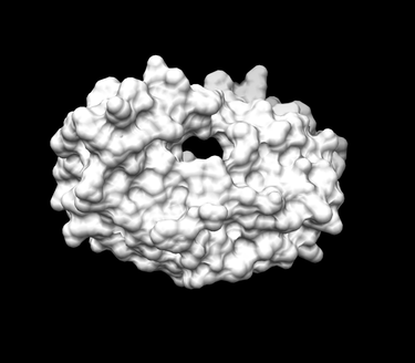
Generating the Receptor Surface
Check to make sure 02.surface-spheres directory exists under dock-tutorial. If not then make the following directory:
mkdir 02.surface-sphgen
cd 02.surface-sphgen
The following steps will be carried out to generate the receptor surface using Chimera:
Open Chimera by simply typing chimera into the terminal window
| Go File -> Open and choose the PDB file of the protein containing no hydrogens (1HVR.receptor.noH.pdb) from 01.dockprep
| Further, Actions -> Surface -> Show
| Go Tools -> Structure Editing -> Write DMS in order to obtain a dms file, which we will need to place spheres
| In the new window save the surface as 1HVR.receptor.dms
Placing Spheres
We will be using SPHGEN to generate spheres: see the DOCK online owners manual for additional information:
<http://dock.compbio.ucsf.edu/DOCK_6/dock6_manual.htm>
The following steps will be used to place the spheres on the receptor surface:
1. Create a file called INSPH and fill it out as follows, then save it. This input file tells SPHGEN what to do, details of each line are below:
1HVR.receptor.dms
R
X
0.0
4.0
1.4
1HVR.receptor.sph
Input File Details:
 1HVR.receptor.dms - surface file from the previous step
 R - tells SPHGEN to place spheres either outside of the surface (R) or inside the surface (L)
 X - tells SPHGEN the subset of surface points to be used (X=all points)
 0.0 - prevents generation of large spheres with close surface contacts(defalut=0.0)
 4.0 - maximum sphere radius in angstroms (default=4.0)
 1.4 - minimum sphere radius in angstroms (default=radius of probe)
 1HVR.receptor.sph - clustered spheres file that we want to generate
2. Run the sphgen program from the terminal:
sphgen -i INSPH -o OUTSPH
-i tells sphgen where the input file INSPH is
INSPH tells sphgen what to do
-o tells sphgen what to call the oputput file
OUTSPH is the output file containing the sphere information
3. (optional) To look at the spheres generated, you need to put them into PDB format.
Run showsphere, by typing the follwoing into the terminal:
showsphere
You will be prompted with the following questions:
Enter name of sphere cluster file:
     1HVR.receptor.sph
Enter cluster number to process (<0 = all):
     -1
Generate surfaces as well as pdb files (<N>/Y)?
     N
Enter name for output file prefix:
     output_spheres
Process cluster 0 (contains ALL spheres) (<N>/Y)?
     N
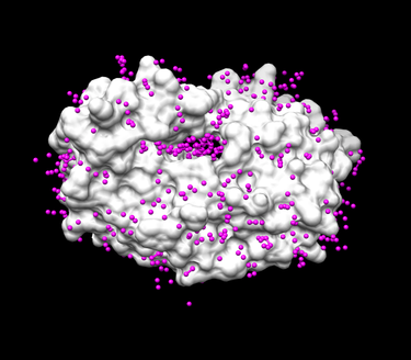
You can then open the receptor file in Chimera as well as the output_spheres.pdb file and should see many spheres placed all over the receptor surface.
4. Run the sphere_selector program from in the terminal to select spheres of interest (note: not all of the spheres in the previous image are in the active site so we want to eliminate them):
sphere_selector 1HVR.receptor.sph ../01.dockprep/1HVR.ligand.mol2 8.0
This program goes to select the spheres within a user-defined radius (8.0 here) of a target molecule from a previously obtained file: 1HVR.receptor.sph. In turn, a new file selected_spheres.sph will be generated.
5. Run showsphere to visualize the spheres:
showsphere
When prompted on the command line, answering the questions as follows:
Enter name of sphere cluster file:
     selected_spheres.sph
Enter cluster number to process (<0 = all):
     -1
Generate surfaces as well as pdb files (<N>/Y)?
     N
Enter name for output file prefix:
     output_spheres_selected
Process cluster 0 (contains ALL spheres) (<N>/Y)?
     N
- Launch Chimera, choose File -> Open, choose 1HVR.receptor.noH.pdb
- Go File -> Open, choosing output_spheres_selected.pdb
- Go Select -> Residue -> SPH
- Finally, Actions -> Atoms/Bonds -> sphere
The final image should look similar to the example below:
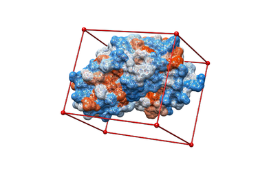
IV. Generating Box and Grid
Mosavverul Arkin
- 1 Make a new directory and name it: 03.box-grid/
mkdir 03.box-grid
- 2 Make a new file in this directory and name it showbox.in
vim showbox.in
- 3 This will automatically open the file showbox.in. Edit the file showbox.in as follows:
   Y                                               #Yes, generate a box
   8.0                                             #Size of the box in Angstroms
   ../02.surfaces-spheres/selected_spheres.sph     #Sphere.sph file
   1                                               #Cluster number
   1HVR.box.pdb                                    #Name of the output file
- 4 Save the file by the inputting the command:
:wq
- 5 Run the command:
showbox < showbox.in
- 6 Make a new file in the same directory (03.box-grid/) and name it: grid.in
vim grid.in
This will automatically open the file grid.in. Edit this file with the following parameters:
    compute_grids                   yes                  # compute scoring grids (yes)
    grid_spacing                      0.4                  # what is the distance between grid points along each axis (in Angstroms).
    output_molecule                no                   # write up coordinates of the receptor into a new file
    contact_score                     no                   # compute contact grid? default is no
    energy_score                      yes                  # compute energy score? yes - we are using this method to compute force fields on probes
    energy_cutoff_distance       9999               # the max distance between atoms for the energy contribution to be computed
    atom_model                       a                     # atom_model u means united atom model where atoms are attached to hydrogens, and a stands for all-atom model, where                                                                  hydrogens on carbons are treated separately
    attractive_exponent           6                     #attractive component stands for exponent of the attractive LJ term in VDW potential
    repulsive_exponent            9                     #repulsive component stands for exponent in the repulsive LJ term in VDW potential
    distance_dielectric             yes
    dielectric_factor                 4
    bump_filter                       yes
    bump_overlap                   0.75
    receptor_file                      ../01.dockprep/1HVR.receptor.mol2
box_file 1HVR.box.pdb
vdw_definition_file ../00.files/vdw_AMBER_parm99.defn
score_grid_prefix 1HVR.grid
distance dielectric stands for the dielectric constant to be linearly dependent on distance distance dielectric factor is the coefficient of the dielectric bump filter flag determines if we want to screen orientation for clashes before scoring and minimization bump_overlap stands for the fraction of allowed overlap where 1 corresponds to no allowed overlap and 0 corresponds to full overlap being permitted. our receptor file the box file we generated in the Box section VDW parameters file Prefix for the grid file name. All the extensions will be generated automatically.
V. Docking a Single Molecule for Pose Reproduction
Rigid Ligand DOCKing
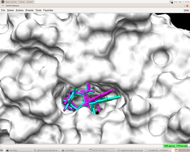
Rigid Ligand Docking is usually used to check the validity of docking program and user-defined parameters because it's much faster than flexible docking. It also helps users to identify any mistakes made during the preparation of receptor and ligand. In our case, we know the experimental structure of a receptor-ligand complex. So if we dock the ligand back to the ligand-free receptor. The pose predicted by DOCK should be very close to the experimental one. Otherwise, users should examine the parameters and all the files involved.
Here is the input for DOCK6
  ligand_atom_file                                             ../01.dockprep/1HVR.ligand.mol2
  limit_max_ligands                                            no
  skip_molecule                                                no
  read_mol_solvation                                           no
  calculate_rmsd                                               yes
  use_rmsd_reference_mol                                       yes
  rmsd_reference_filename                                      ../01.dockprep/1HVR.ligand.mol2
  use_database_filter                                          no
  orient_ligand                                                yes
  automated_matching                                           yes
  receptor_site_file                                           ../02.surface-spheres/selected_spheres.sph
  max_orientations                                             1000
  critical_points                                              no
  chemical_matching                                            no
  use_ligand_spheres                                           no
  use_internal_energy                                          no
  flexible_ligand                                              no
  bump_filter                                                  no
  score_molecules                                              yes
  contact_score_primary                                        no
  contact_score_secondary                                      no
  grid_score_primary                                           yes
  grid_score_secondary                                         no
  grid_score_rep_rad_scale                                     1
  grid_score_vdw_scale                                         1
  grid_score_es_scale                                          1
  grid_score_grid_prefix                                       ../03.box-grid/1HVR.grid
  multigrid_score_secondary                                    no
  dock3.5_score_secondary                                      no
  continuous_score_secondary                                   no
  descriptor_score_secondary                                   no
  gbsa_zou_score_secondary                                     no
  gbsa_hawkins_score_secondary                                 no
  SASA_descriptor_score_secondary                              no
  amber_score_secondary                                        no
  minimize_ligand                                              yes
  simplex_max_iterations                                       1000
  simplex_tors_premin_iterations                               0
  simplex_max_cycles                                           1
  simplex_score_converge                                       0.1
  simplex_cycle_converge                                       1.0
  simplex_trans_step                                           1.0
  simplex_rot_step                                             0.1
  simplex_tors_step                                            10.0
  simplex_random_seed                                          0
  simplex_restraint_min                                        yes
  simplex_coefficient_restraint                                10.0
  atom_model                                                   all
  vdw_defn_file                                                ../03.box-grid/vdw_AMBER_parm99.defn
  flex_defn_file                                               ../00.files/flex.defn
  flex_drive_file                                              ../00.files/flex_drive.tbl
  ligand_outfile_prefix                                        1HVR.out
  write_orientations                                           no
  num_scored_conformers                                        100
  write_conformations                                          no
  cluster_conformations                                        no
  rank_ligands                                                 no
Note that "flexible_ligand" is turned off. "minimize_ligand" has to be on.
The predicted pose and the experimental pose have an RMSD less than 2.000 which means the prediction reproduced the result from experiment.
Flexible Ligand DOCKing
In the case of flexible ligand DOCKing, the ligand is allowed to be flexible. This type of docking allows the ligand to structurally rearrange in response to the receptor. Initially the largest rigid substructure of the ligand is identified; then the flexible layers are identified. The orientations are ranked according to their score, and are grouped by root mean squared deviation (RMSD). To run the docking calculation, use the program dock6 that is distributed with DOCK in the /bin directory. You need to generate an input file by answering questions interactively or manually via text file. The program will generate an output file summarizing the parameters used in the run, any warning or error messages, and summary information about the best scoring pose. It will also produce a structure (.mol2) file, containing the geometric coordinates of the best pose as well as a summary of the interaction energy of that pose.
VI. Virtual Screening
Virtual Screening Introduction
Virtual screening is a method used to predict most favorable ligand binding to a target protein within a ligand database. It also allows for comparison of both qualitative (e.g. position in binding site) and quantitative (e.g. grid scores, internal energy) data pertaining to the each screened ligand with the originally docked molecule.
To perform virtual screening, HIVPR.ligands.005.mol2, a mol2 file that contains 5 small molecules will be the virtual library based on the receptor 1HVR. This is a reasonable computational cost for a quick search, so we can conduct it on our own computer. After that, virtual screening can be conducted within a larger database, HIVPR.ligands.100.mol2, which contains 100 ligands. Since the computational cost of virtual screening is much higher, it is better for us to run it on Seawulf.
Running Virtual Screening
Before running virtual screening, a new directory 05.mini-virtual-screen is created and ligand files HIVPR.ligands.005.mol2 and HIVPR.ligands.100.mol2 are copied from Wjallen. Since most parameters of dock.in and new virtual screening input are the same, we can make few modifications to dock.in script but rename it as mini-virtual-screen.in.
  mkdir 05.mini-virtual-screen
  cd 05.mini-virtual-screen
  cp ~wjallen/AMS536/multi-mol2/files/HIVPR.ligands.005.mol2 ./
  cp ../04.dock/dock.in/ ./
  mv dock.in mini-virtual-screen.in
Here is the content of mini-virtual-screen.in
  ligand_atom_file                                             HIVPR.ligands.005.mol2
  limit_max_ligands                                            no
  skip_molecule                                                no
  read_mol_solvation                                           no
  calculate_rmsd                                               no
  use_database_filter                                          no
  orient_ligand                                                yes
  automated_matching                                           yes
  receptor_site_file                                           ../02.surface-spheres/selected_spheres.sph
  max_orientations                                             1000
  critical_points                                              no
  chemical_matching                                            no
  use_ligand_spheres                                           no
  use_internal_energy                                          yes
  internal_energy_rep_exp                                      12
  flexible_ligand                                              yes
  user_specified_anchor                                        no
  limit_max_anchors                                            no
  min_anchor_size                                              5
  pruning_use_clustering                                       yes
  pruning_max_orients                                          1000
  pruning_clustering_cutoff                                    100
  pruning_conformer_score_cutoff                               100
  use_clash_overlap                                            no
  write_growth_tree                                            no
  bump_filter                                                  no
  score_molecules                                              yes
  contact_score_primary                                        no
  contact_score_secondary                                      no
  grid_score_primary                                           yes
  grid_score_secondary                                         no
  grid_score_rep_rad_scale                                     1
  grid_score_vdw_scale                                         1
  grid_score_es_scale                                          1
  grid_score_grid_prefix                                       ../03.box-grid/1HVR.grid
  multigrid_score_secondary                                    no
  dock3.5_score_secondary                                      no
  continuous_score_secondary                                   no
  descriptor_score_secondary                                   no
  gbsa_zou_score_secondary                                     no
  gbsa_hawkins_score_secondary                                 no
  SASA_descriptor_score_secondary                              no
  amber_score_secondary                                        no
  minimize_ligand                                              yes
  minimize_anchor                                              yes
  minimize_flexible_growth                                     yes
  use_advanced_simplex_parameters                              no
  simplex_max_cycles                                           1
  simplex_score_converge                                       0.1
  simplex_cycle_converge                                       1.0
  simplex_trans_step                                           1.0
  simplex_rot_step                                             0.1
  simplex_tors_step                                            10.0
  simplex_anchor_max_iterations                                500
  simplex_grow_max_iterations                                  1000
  simplex_grow_tors_premin_iterations                          0
  simplex_random_seed                                          0
  simplex_restraint_min                                        no
  atom_model                                                   all
  vdw_defn_file                                                ../00.files/vdw_AMBER_parm99.defn
  flex_defn_file                                               ../00.files/flex.defn
  flex_drive_file                                              ../00.files/flex_drive.tbl
  ligand_outfile_prefix                                        1HVR.output
  write_orientations                                           no
  num_scored_conformers                                        100
  rank_ligands                                                 no
Analyzing the Results
After conducting virtual screening on local machine, a file named 1HVR.output_scored.mol2 is obtained, which contains successfully docked ligands, including grid score, internal energy, etc and it looks like this:
  ##########           Name:		NONAME
  ##########    Grid Score:          -25.904999
  ##########      Grid_vdw:          -25.904999
  ##########         Grid_es:            0.000000
  ##########    Int_energy:            0.062399
  @<TRIPOS>MOLECULE
  NONAME
  20 20 1 0 0
  SMALL
  NO_CHARGES
  @<TRIPOS>ATOM
     1 O          -6.5962   19.4021   23.0405 O.2     1  <1>         0.0000
     2 C          -6.8355   18.4953   22.2343 C.2     1  <1>         0.0000
     3 N          -7.8272   17.5802   22.4935 N.am    1  <1>         0.0000
     4 H          -8.3181   17.7085   23.3731 H       1  <1>         0.0000
     5 C          -8.2659   16.4500   21.6933 C.3     1  <1>         0.0000
     6 H          -9.1047   15.9926   22.2333 H       1  <1>         0.0000
     7 H          -7.4773   15.6904   21.6784 H       1  <1>         0.0000
     8 C          -8.7214   16.8444   20.2915 C.3     1  <1>         0.0000
     9 H          -9.4627   17.6481   20.3875 H       1  <1>         0.0000
    10 O          -9.4130   15.7379   19.7151 O.3     1  <1>         0.0000
    11 H         -10.1762   15.5384   20.2849 H       1  <1>         0.0000
    12 C          -7.5968   17.3421   19.3635 C.3     1  <1>         0.0000
    13 H          -7.8639   18.3502   19.0239 H       1  <1>         0.0000
    14 O          -7.5032   16.5445   18.1836 O.3     1  <1>         0.0000
    15 H          -8.3854   16.5076   17.7791 H       1  <1>         0.0000
    16 C          -6.2182   17.4085   20.0113 C.3     1  <1>         0.0000
    17 H          -5.4732   17.6806   19.2547 H       1  <1>         0.0000
    18 H          -5.8956   16.4394   20.4044 H       1  <1>         0.0000
    19 N          -6.1245   18.4045   21.0622 N.am    1  <1>         0.0000
    20 H          -5.4272   19.1287   20.9184 H       1  <1>         0.0000
  @<TRIPOS>BOND
    1     1     2    2
    2     2     3   am
    3     2    19   am
    4     3     4    1
    5     3     5    1
    6     5     6    1
    7     5     7    1
    8     5     8    1
    9     8     9    1
   10     8    10    1
   11     8    12    1
   12    10    11    1
   13    12    13    1
   14    12    14    1
   15    12    16    1
   16    14    15    1
   17    16    17    1
   18    16    18    1
   19    16    19    1
   20    19    20    1
After running virtual screening in Seawulf, we will get 1HVR.output_scored.mol2 which contains the mol2 files of all successfully docked ligands, virtual_screen.out file which contains the dock results of successfully docked ligands, and virtual_screen.out.1 to virtual_screen.out.3 which contain dock results from different nodes you use (the number is related with the number of nodes you use, here we use 4 nodes).
Molecule: CHEMBL171551
   Anchors:               3
   Orientations:          3000
   Conformations:         359
       Grid Score:          -60.092117
        Grid_vdw:          -62.332535
           Grid_es:            2.240418
      Int_energy:           13.718960
These files should copied to local computers if we want to use Chimera to visually check the results. In Seawulf, move to 06.virtual-screen/ directory,
Scp –r yanxie@herbie.mathlab.sunysb.edu:~/AMS536/dock_tutorial/
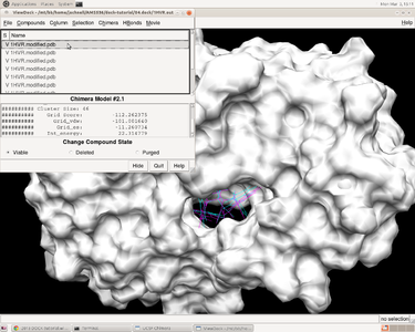
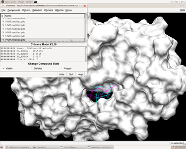
In herbie, open the receptor 1HVR.receptor.mol2 and reference ligand 1HVR.ligand.mol2 in 01.dockprep/ directory and then we can check how the ligands fitting the receptor by ViewDock function in Chimera. Go to Tools -> Surface/Binding Analysis -> ViewDock and choose 1HVR.output_scored.mol2.In the pup-up window, you can go to Column ->show -> Grid Score to show the grid score, and then you can click on the head of the column to rank order all the ligands by their grid scores. and the reference ligand is colored according to elements. As you can see, the best scored ligand fits in the binding pocket very well, but the worst scored one almost sticks out of the binding pocket.
VII. Running DOCK in Parallel on Seawulf
The Seawulf Cluster is a custom-built 470-processor (235 dual processor nodes and 2 processors per node) Linux Cluster capable of highly parallel processing. It severs as to provide computational resources and expertise for basic scientific research to the faculty and students of Stony Brook University.
Typically, to dock one ligand, one processor on a single node will be used, while for docking multiple ligands, more than one processor can be used in parallel mode. However, the number of processors used should be less than the number of ligands for dock.
Before running DOCK on Seawulf, we need to copy our whole dock-tutorial files from Herbie to Seawulf. Log into the Seawulf through Herbie, and then type,
scp -r username@herbie.mathlab.sunysb.edu:~/AMS536/dock-tutorial/ ~/AMS536/
First, making a file named qsub.csh with the following context,
 #!/bin/csh
 #PBS -l nodes=2:ppn=2
 #PBS -l walltime=10:00:00
 #PBS -N 1HVR.vs
 #PBS -o 1HVR.output
 #PBS -j oe
 #PBS –V

 cd /nfs/user03/username/AMS536/dock-tutorial/06.virtual-screen
 mpirun -np 4 /nfs/user03/wjallen/local/dock6/bin/dock6.mpi -i virtual_screen.in -o virtual_screen.out
Explanation of the commands,
#!/bin/csh: Execute script with tcsh
#PBS -l nodes=2:ppn=2: Use 2 nodes, and 2 processors per node, so 4 processors
#PBS -l walltime=10:00:00: Allow 10 hours for your job run
#PBS -N 1HVR.vs: Name of your job
#PBS -o 1HVR.output: Name of your output file
#PBS -j oe: Combine the output and error streams into a single output file
#PBS –V: Show more information about what is happening for the users
cd /nfs/user03/username/AMS536/dock-tutorial/06.virtual-screen: Change to your home directory and folder with dock files
mpirun -np 4 /nfs/user03/wjallen/local/dock6/bin/dock6.mpi -i virtual_screen.in -o virtual_screen.out: This line specifies path to dock executable and provide input and output filenames. Notice that in order to run DOCK in parallel (on 4 processors here), we need to use dock6.mpi instead of dock6. Message passing interface ( MPI) is basically a program that allows programs like DOCK to run in parallel.
Then, we can run the dock virtual screen on Seawulf by submitting the DOCK experiment to the Seawulf queue,
qsub virtual_screen.in
You can use the command qstat to show the status of pbs batch jobs,
 qstat #the whole list of submitted jobs in queue

 qatat-u username #the whole list of jobs in queue you submitted
For more information, see PBS Queue.
VIII. Frequently Encountered Problems
You should always be clear about what the input file and output file of one program are and what format they are. Sometimes, it's easy to make mistakes if you are confused about which direction you are, so make sure you know that all the time.
Mike
The most common problem experienced in UNIX is having the wrong file path. ALWAYS CHECK TO MAKE SURE THAT YOUR FILE PATH IS CORRECT This can be facilitated with the Tab button which will auto complete what you have started to type.
Ivan
Make sure you are opening the correct files for each visualization step (e.g. opening the receptor file with the ligand still there may make analyzing your docking results a bit more challenging).
Use the auto-fill (tab) function but double check to make sure the correct file was auto-filled (e.g. if you type 1H then hit tab you might get 1HVR_selected_spheres but the file you want actually is 1HVR_selected_spheres.sph).
Junjie
Kai
For users with no UNIX experience and limited programming experience - it's a good idea to run through a couple tutorials before you start using UNIX. Even if you type in the commands without fully understanding their implications, become familiar with the basic commands and shortcuts. It will help a lot when you actually start using UNIX!
Arkin
Yan
Yao
Lu
Fengfei
Mosavverul
Joe
Write some text here..
command or input file
