2021 DOCK tutorial 3 with PDBID 1S19
Contents
Introduction
DOCK
Developed by Irwin D. Kuntz, Jr. and colleagues at UCSF, DOCK is a program used to dock molecules to one another. Docking is a process in which given a small molecule or ligand in the active site of a receptor, the program will try to predict the lowest-energy binding mode of the ligand to the receptor. This process is very important in drug discovery as small molecules that bind to or interact with the active site of a receptor associated with a disease could inhibit its function, acting as a drug. DOCK is a particularly helpful tool as it is used to screen massive libraries of molecules, containing millions of compounds, against a receptor to identify the most promising drug lead compounds.
DOCK historically used a geometric matching algorithm to superimpose the ligand onto a negative image of the active site of the receptor. Over the years, features were added that would improve the programs ability to find the lowest-energy binding mode. Somem of these features include force-field based scoring, on-the-fly optimization and an algorithm for flexible ligand docking.
In this tutorial DOCK6 will be used. New features for DOCK6 include: additional scoring options during minimization; DOCK 3.5 scoring-including Delphi electrostatics, ligand conformational entropy corrections, ligand desolvation, receptor desolvation; Hawkins-Cramer-Truhlar GB/SA solvation scoring with optional salt screening and more (see UCSF DOCK). These new features improved the programs ability to predict binding poses.
1S19
This tutorial will use PDB code: 1S19. 1S19 is the crystal structure of VDR ligand binding domain complexed to calcipotriol (find structure here. The resolution is 2.10 Å.
Chimera
UCSF Chimera was developed by Resource for Biocomputing, Visualization, and Informatics (RBVI) at the University of California, San Francisco. Chimera is a program made for the interactive visualization and analysis of molecular structures. Some features of Chimera include general structure analysis (automatic identification of an atom, hydrogen addition and partial charge assignment, structure building and bond rotation, etc.) presenting images and movies (high-res images, visual effects, standard molecular representations, etc.) and sequence structure tools (sequence alignments, structure superposition, etc.)
Making Directories
To make it easier for us to locate certain files, we are going to create directories for each step of the docking process. The mkdir command creates a new directory in which new files can be saved. The cd command allows for you to navigate between directories.
In your Bash Shell environment, create a directory containing all of the information for the project by typing:
mkdir 1S19
To change into that directory type:
cd 1S19
To create the directories for each step:
mkdir 001.structure 002.surface_spheres 003.gridbox 004.dock 005.virtual_screen 006.virtual_screen_mpi 007.cartesianmin 008.rescore
To confirm that the directories have been created:
ls
If you made a mistake and need to delete a directory:
rm *insert name of directory to be deleted*
Preparing the Ligand and Receptor
PDB Structure
Download the structure of 1S19 from the Protein Data Bank (PDB).
Download Files -> PDB Format
This file contains the coordinates for the 3D structure of the receptor, ligand and any other molecules present during the experiment (typically water or metal ions). To visualize the structure, we will be using Chimera.
Visualization with Chimera To open the newly downloaded PDB coordinates:
File -> Open
The protein when you first open the file should look like the image below. You can change the view of the structure by rotating it with your mouse or touchpad. Currently, some of the side chains of the backbone are shown, there are no hydrogens or partial charges, and there are some water molecules present.
Receptor
In order to dock, the ligand and receptor have to be separated and saved into different files. To do this is a simple process and can be done in Chimera. To hide all sidechain bonds:
  Select -> standard amino acids
  Actions -> Atoms/Bonds -> hide
To prepare the receptor, we are going to want to delete everything except the protein from the PDB file. To do this in Chimera:
  Select -> Residue -> All nonstandard
  Actions -> Atoms/Bonds -> Delete
You will now be left with only the desired protein. To save this file, we are going to save it as a mol2 file. This can be done by:
File -> Save Mol2 -> "1s19_receptor_woH.mol2"
Adding Hydrogens and Charge PDB structures are reported without hydrogens, so it is important that we add them to the receptor in order to gain accurate calculations for the interactions between the protein and ligand. This can also be done in Chimera by doing the following:
Tools -> Structure Editing -> Add H -> Ok
We will also need to add charges to the receptor
Tools -> Structure Editing -> Add Charge -> (have Amber ff14SB and AM1-BCC selected) -> Ok
Once this is done it is very important to check that the charges of the receptor match that of the experiments. Chimera adds the standard protonation states to the amino acids, so it's important to read the paper associated with the PDB file (see here) to make sure that there are no amino acids that are specifically protonated or deprotonated.
Once you have checked to make sure that the protonation states are okay, save this as a mol2 file:
File -> Save Mol2 -> "1s19_receptor_dockprep.mol2"
Ligand
Like the receptor, we will need to save the ligand as a separate mol2 file in order to perform the docking. For this model, the ligand is named as MC9 in Chimera.
To isolate the ligand:
  Select -> Residue -> MC9
  Select -> Invert (all models)
  Actions -> Atoms/Bonds -> Delete
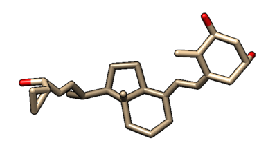
We are now left with just the ligand as pictured below.
We will save this as a mol2 file by:
File -> Save Mol2 -> 1s19_lig_woH.mol2
Adding Hydrogens and Charges In the same steps as the receptor, we will add hydrogens and partial charges to the ligand. For the Hydrogens:
Tools -> Structure Editing -> Add H
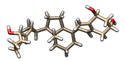
After doing so, the structure should look like the one below.
Now we have to add the charges to the ligand. Remember to double check the crystal structure and validate the charge. In this case the charge is neutral (+/- 0), and Chimera was able to model it correctly. However this is not always the case and you will sometimes be required to manually change the charges.
Save this final structure as a mol2 file with the name "1s19_lig_dockprep.mol2"
Generating Receptor Surface and Spheres
Generating Surface
In Chimera we can generate a representation of the receptor that creates a negative image of the protein. This surface will guide the ligand to the active site of the receptor during docking. To do this, we are going to open the receptor without hydrogens in Chimera, 1s19_receptor_woH.mol2. Then in Chimera, do:
  Actions -> Surface -> Show
  Tools -> Structure Editing -> Write DMS -> "1s19_rec_surface.dms"
Move this to the "002.surface_spheres" directoy in the Bash Shell environment. THe following Figure is the depiction of the surface in Chimera.
Generating Spheres
Spheres in docking represent empty space in the receptor. Now that we have the surface representation of our receptor, we are going to use the sphgen ("sphere generation") script to create the largest possible sphere for any given empty space. It is okay that spheres overlap with each other, however we do not want any spheres overlapping with the protein.
Still in the "002.surface_spheres" directory, we are going to create a file calle INSPH (short for "in spheres"). To do this type:
vim INSPH
In this new file, we are going to write a script in order to automate the process of generating the spheres. Below is an example of the script that we used.
  1s19_rec_surface.dms    # your receptor as DMS file
  R                       # <R flag> - enables sphere generation outside the protein surface (no eclipsing)
  X                       # <X flag  - uses all coordinates
  0.0                     # <double> - distance that steric interactions are checked
  4.0                     # <double> - Maximum sphere radius of generated sphere
  1.4                     #  <double> - Size of sphere that rolls over dms file surface for cavities
  1s19_receptor_woH.sph   # the name of your output file
With this script saved, you can now run it through sphgen by the following:
sphgen -i INSPH -o OUTSPH
When this is run, the program will generate the "1s19_receptor_woH.sph" file and also an "OUTSPH" file. Looking at 1s19_receptor_woH.sph in Chimera will give you the following image.
Selecting Spheres We are more concerned with the empty space near the active site of the receptor, since that is where we are going to be docking our ligand. To only select particular spheres within 10 angstroms of the ligand, we executed the following command:
sphere_selector 3vjk_receptor_woH.sph 3vjk_ligand_H.mol2 10.0
This generated a new file called "selected_spheres.sph" in our working directory. The result of the sphere selection is show in the image below.
Creating Box and Grid
To make the amount of calculations we have to do smaller, and thus more efficient, we will create a grid in which relevent residues/atoms are selected. This method of creating the box and grid will eliminate any long-distance interactions that the ligand may have.
Generating Box
We will create the box by using the Showbox program. To do this, we will create the following file in our "003.gridbox" directory.
vim showbox.in
We put the following script inside the showbox.in file:
  Y                                           #generate box#
  8.0                                         #how many angstroms the box edges should be from the spheres
  ./../002.surface_spheres/select_spheres.sph #the location of the selected spheres
  1
  1s19.box.pdb                                #name of the output file
To execute this script, type the following:
showbox < showbox.in
Once this program has run, the 1s19.box.pdb file should be in the working directory.
Generating Grid
Next, we will be generating the grid. To do so, we will create a file called grid.in
vim grid.in
The following script will be copied into the grid.in file
  compute_grids                             yes
  grid_spacing                              0.4
  output_molecule                           no
  contact_score                             no
  energy_score                              yes
  energy_cutoff_distance                    9999
  atom_model                                a
  attractive_exponent                       6
  repulsive_exponent                        9
  distance_dielectric                       yes
  dielectric_factor                         4.
  bump_filter                               yes
  bump_overlap                              0.75
  receptor_file                             ./../001.structure/1s19_receptor_dockprep.mol2
  box_file                                  1s19.box.pbd
  vdw_definition_file                       /gpfs/projects/AMS536/zzz.programs/dock6.9_release/parameters/vdw_AMBER_parm99.defn
  score_grid_prefix                         grid
To run this script, type:
grid -i grid.in -o gridinfo.out
When this program finishes running, you should have three new files: gridinfo.out, grid.nrg, and grid.bmp
Energy Minimization
The ligand pose in the crystal structure may not accurately represent the lowest energy conformation of the ligand in a biological system. Therefore, to accurately dock the ligand, we first need to reduce the overall potential energy of the ligand to its global minimum. To do this, we are going to create an energy minimization script:
vim min.in
We used the following script for the minimizaiton:
 conformer_search_type                                        rigid
 use_internal_energy                                          yes
 internal_energy_rep_exp                                      12
 internal_energy_cutoff                                       100.0
 ligand_atom_file                                             ./../001.build/1s19_ligand_dockprep.mol2
 limit_max_ligands                                            no
 skip_molecule                                                no
 read_mol_solvation                                           no
 calculate_rmsd                                               yes
 use_rmsd_reference_mol                                       yes
 rmsd_reference_filename                                      ./../001.build/1s19_ligand_dockprep.mol2
 use_database_filter                                          no
 orient_ligand                                                no
 bump_filter                                                  no
 score_molecules                                              yes
 contact_score_primary                                        no
 contact_score_secondary                                      no
 grid_score_primary                                           yes
 grid_score_secondary                                         no
 grid_score_rep_rad_scale                                     1
 grid_score_vdw_scale                                         1
 grid_score_es_scale                                          1
 grid_score_grid_prefix                                       ./../003.gridbox/grid
 multigrid_score_secondary                                    no
 dock3.5_score_secondary                                      no
 continuous_score_secondary                                   no
 footprint_similarity_score_secondary                         no
 pharmacophore_score_secondary                                no
 descriptor_score_secondary                                   no
 gbsa_zou_score_secondary                                     no
 gbsa_hawkins_score_secondary                                 no
 SASA_score_secondary                                         no
 amber_score_secondary                                        no
 minimize_ligand                                              yes
 simplex_max_iterations                                       1000
 simplex_tors_premin_iterations                               0
 simplex_max_cycles                                           1
 simplex_score_converge                                       0.1
 simplex_cycle_converge                                       1.0
 simplex_trans_step                                           1.0
 simplex_rot_step                                             0.1
 simplex_tors_step                                            10.0
 simplex_random_seed                                          0

 simplex_restraint_min                                        yes
 simplex_coefficient_restraint                                10.0
 atom_model                                                   all
 vdw_defn_file
 /gpfs/projects/AMS536/zzz.programs/dock6.9_release/parameters/vdw_AMBER_parm99.defn
 flex_defn_file
 /gpfs/projects/AMS536/zzz.programs/dock6.9_release/parameters/flex.defn
 flex_drive_file
 /gpfs/projects/AMS536/zzz.programs/dock6.9_release/parameters/flex_drive.tbl
 ligand_outfile_prefix                                        1s19.lig.min
 write_orientations                                           no
 num_scored_conformers                                        1
 rank_ligands                                                 no
Now that the script is made, we can run the energy minimization by the following line
dock6 -i min.in -o min.out
Running this command will yield two new files in the direectory: min.out and 1s19.lig.min_scored.mol2
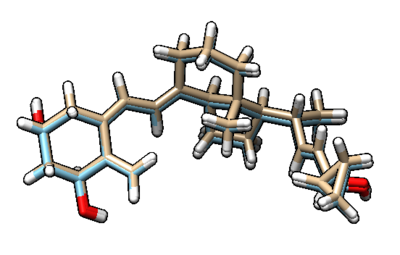
You can visualize the minimized ligand and the original ligand in Chimera to observe the difference between the two.
The beige structure is the minimized ligand and the blue structure is the original ligand. The difference between the two is not large. To see the RMSD (room mean squared deviation) between the two, you can vim into the 1s19.lig.min_scored.mol2 file that was generated. The picture below shows the top of that file, and RMSD between the two molecules is 0.2281.
Footprint Analysis
We can use the moleucular footprint to understand the lignad binding to the receptor by using electrostatic and Van der Waals interactions. We will be doing footprint analysis for our minimization of the ligand and also the rigid, flex, and fixed anchor docking. To begin this analysis, create the file footprint.in and copy the following script into the file:
conformer_search_type                                        rigid
use_internal_energy                                          no
ligand_atom_file                                             ./../004.dock/1s19.lig.min_scored.mol2
limit_max_ligands                                            no
skip_molecule                                                no
read_mol_solvation                                           no
calculate_rmsd                                               no
use_database_filter                                          no
orient_ligand                                                no
bump_filter                                                  no
score_molecules                                              yes
contact_score_primary                                        no
contact_score_secondary                                      no
grid_score_primary                                           no
grid_score_secondary                                         no
multigrid_score_primary                                      no
multigrid_score_secondary                                    no
dock3.5_score_primary                                        no
dock3.5_score_secondary                                      no
continuous_score_primary                                     no
continuous_score_secondary                                   no
footprint_similarity_score_primary                           yes
footprint_similarity_score_secondary                         no
fps_score_use_footprint_reference_mol2                       yes
fps_score_footprint_reference_mol2_filename                  ./../001.structure/1s19_ligand_dockprep.mol2
fps_score_foot_compare_type                                  Euclidean
fps_score_normalize_foot                                     no
fps_score_foot_comp_all_residue                              yes
fps_score_receptor_filename                                  ./../001.structure/1s19_dockprep.mol2
fps_score_vdw_att_exp                                        6
fps_score_vdw_rep_exp                                        9
fps_score_vdw_rep_rad_scale                                  1
fps_score_use_distance_dependent_dielectric                  yes
fps_score_dielectric                                         4.0
fps_score_vdw_fp_scale                                       1
fps_score_es_fp_scale                                        1
fps_score_hb_fp_scale                                        0
pharmacophore_score_secondary                                no
descriptor_score_secondary                                   no
gbsa_zou_score_secondary                                     no
gbsa_hawkins_score_secondary                                 no
SASA_score_secondary                                         no
amber_score_secondary                                        no
minimize_ligand                                              no
atom_model                                                   all
vdw_defn_file                                               /gpfs/projects/AMS536/zzz.programs/dock6.9_release/parameters/vdw_AMBER_parm99.defn
flex_defn_file                                               /gpfs/projects/AMS536/zzz.programs/dock6.9_release/parameters/flex.defn
flex_drive_file                                              /gpfs/projects/AMS536/zzz.programs/dock6.9_release/parameters/flex_drive.tbl
ligand_outfile_prefix                                        footprint.out
write_footprints                                             yes
write_hbonds                                                 yes
write_orientations                                           no
num_scored_conformers                                        1
rank_ligands                                                 no
To run the script, type the following:
dock6 -i footprint.in
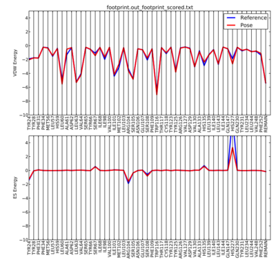
To visualize the footprint, we can run a python script that will plot the results for us.
With this script in our directory, we can run it by the following line. The 50 at the end of the line denotes that we are going to be plotting the distribution of the 50 most significant residues.
python plot_footprint_single_magnitude.py footprint.out_footprint_scored.txt 50
The output plot from the python script should look like the picture below.
This process was done for the minimized ligand. However, after following the next three docking steps in the tutorial, you can repeat the footprint analysis to see the effects that changing the positioning of the ligand has on the protein.
Docking
Rigid Docking
Rigid is the least computationally intensive form of docking - the ligand has no rotational freedom around its bonds and is kept static. The first step is to move to the dock folder and make a folder for rigid docking.
cd 004.dock
mkdir 1S19_rigid
Then we can make an input file for rigid docking and edit in within Vim or the Dock6.9 program.
touch rigid.in
vim rigid.in
Here we will edit the parameters as follows:
conformer_search_type                                        rigid
use_internal_energy                                          yes
internal_energy_rep_exp                                      12
internal_energy_cutoff                                       100
ligand_atom_file                                             ./../004.dock/1S19_lig_min_scored.mol2
limit_max_ligands                                            no
skip_molecule                                                no
read_mol_solvation                                           no
calculate_rmsd                                               yes
use_rmsd_reference_mol                                       yes
rmsd_reference_filename                                      ./../004.dock/1S19_lig_min_scored.mol2
use_database_filter                                          no
orient_ligand                                                yes
automated_matching                                           yes
receptor_site_file                                           ./../002.surface_spheres/selected_spheres.sph
max_orientations                                             1000
critical_points                                              no
chemical_matching                                            no
use_ligand_spheres                                           no
bump_filter                                                  no
score_molecules                                              yes
contact_score_primary                                        no
contact_score_secondary                                      no
grid_score_primary                                           yes
grid_score_secondary                                         no
grid_score_rep_rad_scale                                     1
grid_score_vdw_scale                                         1
grid_score_es_scale                                          1
grid_score_grid_prefix                                       ./../003.gridbox/grid
multigrid_score_secondary                                    no
dock3.5_score_secondary                                      no
continuous_score_secondary                                   no
footprint_similarity_score_secondary                         no
pharmacophore_score_secondary                                no
descriptor_score_secondary                                   no
gbsa_zou_score_secondary                                     no
gbsa_hawkins_score_secondary                                 no
SASA_score_secondary                                         no
amber_score_secondary                                        no
minimize_ligand                                              yes
simplex_max_iterations                                       1000
simplex_tors_premin_iterations                               0
simplex_max_cycles                                           1
simplex_score_converge                                       0.1
simplex_cycle_converge                                       1.0
simplex_trans_step                                           1.0
simplex_rot_step                                             0.1
simplex_tors_step                                            10.0
simplex_random_seed                                          0
simplex_restraint_min                                        no
atom_model                                                   all
vdw_defn_file                                                /gpfs/projects/AMS536/zzz.programs/dock6.9_release/parameters/vdw_AMBER_parm99.defn
flex_defn_file                                               /gpfs/projects/AMS536/zzz.programs/dock6.9_release/parameters/flex.defn
flex_drive_file                                              /gpfs/projects/AMS536/zzz.programs/dock6.9_release/parameters/flex_drive.tbl
ligand_outfile_prefix                                        rigid.out
write_orientations                                           no
num_scored_conformers                                        1
rank_ligands                                                 no
Then we will input the file into Dock6.9 with the following command:
dock6 -i rigid.in
This will output the file rigid.out_scored.mol2, which is visualized in Chimera (blue) over the original minimized ligand (purple).
Fixed Anchor Docking
Fixed docking is the next level up. Here we will keep the major part of the ligand with no rotatable bonds fixed as an anchor but allow rotational freedom around the other rigid groups. Let's begin by making a directory and input file within 004.dock:
cd 004.dock
mkdir 1S19_fixed
cd 1S19_fixed
touch fixed.in
This file can be modified in Vim or in Dock6.9 itself as shown:
conformer_search_type                                        flex
write_fragment_libraries                                     no
user_specified_anchor                                        no
limit_max_anchors                                            no
min_anchor_size                                              5
pruning_use_clustering                                       yes
pruning_max_orients                                          1000
pruning_clustering_cutoff                                    100
pruning_conformer_score_cutoff                               100
pruning_conformer_score_scaling_factor                       1
use_clash_overlap                                            no
write_growth_tree                                            no
use_internal_energy                                          yes
internal_energy_rep_exp                                      12
internal_energy_cutoff                                       100
ligand_atom_file                                             ../../001.structure/1S19_ligand_dockprep.mol2
limit_max_ligands                                            no
skip_molecule                                                no
read_mol_solvation                                           no
calculate_rmsd                                               yes
use_rmsd_reference_mol                                       yes
rmsd_reference_filename                                      ../../001.structure/1S19_ligand_dockprep.mol2
use_database_filter                                          no
orient_ligand                                                no
bump_filter                                                  no
score_molecules                                              yes
contact_score_primary                                        no
contact_score_secondary                                      no
grid_score_primary                                           yes
grid_score_secondary                                         no
grid_score_rep_rad_scale                                     1
grid_score_vdw_scale                                         1
grid_score_es_scale                                          1
grid_score_grid_prefix                                       ../../003.gridbox/grid
multigrid_score_secondary                                    no
dock3.5_score_secondary                                      no
continuous_score_secondary                                   no
footprint_similarity_score_secondary                         no
pharmacophore_score_secondary                                no
descriptor_score_secondary                                   no
gbsa_zou_score_secondary                                     no
gbsa_hawkins_score_secondary                                 no
SASA_score_secondary                                         no
amber_score_secondary                                        no
minimize_ligand                                              yes
minimize_anchor                                              yes
minimize_flexible_growth                                     yes
use_advanced_simplex_parameters                              no
simplex_max_cycles                                           1
simplex_score_converge                                       0.1
simplex_cycle_converge                                       1
simplex_trans_step                                           1
simplex_rot_step                                             0.1
simplex_tors_step                                            10
simplex_anchor_max_iterations                                500
simplex_grow_max_iterations                                  500
simplex_grow_tors_premin_iterations                          0
simplex_random_seed                                          0
simplex_restraint_min                                        no
atom_model                                                   all
vdw_defn_file                                                /gpfs/projects/AMS536/zzz.programs/dock6.9_release/parameters/vdw_AMBER_parm99.defn
flex_defn_file                                               /gpfs/projects/AMS536/zzz.programs/dock6.9_release/parameters/flex.defn
flex_drive_file                                              /gpfs/projects/AMS536/zzz.programs/dock6.9_release/parameters/flex_drive.tbl
ligand_outfile_prefix                                        1S19_fad
write_orientations                                           no
num_scored_conformers                                        100
write_conformations                                          no
cluster_conformations                                        yes
cluster_rmsd_threshold                                       2.0
rank_ligands                                                 no
Upon finishing the 1S19_fixed directory should contain two new output files, fixed.out and 1S19_fad_scored.mol2, which you can open in Chimera as shown.
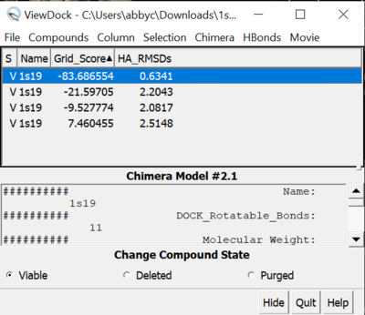
We can also use Chimera to see the calculated properties of the different poses for the ligand. To do this:
  File -> Open -> 2s19_rec_dockprep.mol2
  File -> Open -> 2p16_ligand_dockprep.mol2
  File -> Open -> 1s19_fad_scored.mol2
  Tools -> Surface/binding Analysis -> ViewDock -> 1s19_fad_scored.mol2
  In the loaded dialog box select Dock4,5 or 6
Now you can select which properties of the docking you would like to see. We are going to look at grid scores and RMSDs. To do this:
  Column -> Show -> Gridscore
  Column -> Show -> HA_RMSDs
Flexible Docking
Finally we have the most computationally intensive type of docking, flexible docking, where the ligand has full rotational freedom around its bond angles and all internal degrees of freedom are sampled. Same as before, let's make a directory for the files and write an input file:
cd 004.dock
mkdir 1S19_flexible
cd 1S19_flexible
touch flex.in
Edit the input file in vim or in Dock6.9 itself as follows:
conformer_search_type                                        flex
write_fragment_libraries                                     no
user_specified_anchor                                        no
limit_max_anchors                                            no
min_anchor_size                                              5
pruning_use_clustering                                       yes
pruning_max_orients                                          1000
pruning_clustering_cutoff                                    100
pruning_conformer_score_cutoff                               100
pruning_conformer_score_scaling_factor                       1
use_clash_overlap                                            no
write_growth_tree                                            no
use_internal_energy                                          yes
internal_energy_rep_exp                                      12
internal_energy_cutoff                                       100
ligand_atom_file                                             ../1S19_lig_min_scored.mol2
limit_max_ligands                                            no
skip_molecule                                                no
read_mol_solvation                                           no
calculate_rmsd                                               yes
use_rmsd_reference_mol                                       yes
rmsd_reference_filename                                      ../1S19_lig_min_scored.mol2
use_database_filter                                          no
orient_ligand                                                yes
automated_matching                                           yes
receptor_site_file                                           ../../002.surface_spheres/selected_spheres.sph
max_orientations                                             100
critical_points                                              no
chemical_matching                                            no
use_ligand_spheres                                           no
bump_filter                                                  no
score_molecules                                              yes
contact_score_primary                                        no
contact_score_secondary                                      no
grid_score_primary                                           yes
grid_score_secondary                                         no
grid_score_rep_rad_scale                                     1
grid_score_vdw_scale                                         1
grid_score_es_scale                                          1
grid_score_grid_prefix                                       ../../003.gridbox/grid
multigrid_score_secondary                                    no
dock3.5_score_secondary                                      no
continuous_score_secondary                                   no
footprint_similarity_score_secondary                         no
pharmacophore_score_secondary                                no
descriptor_score_secondary                                   no
gbsa_zou_score_secondary                                     no
gbsa_hawkins_score_secondary                                 no
SASA_score_secondary                                         no
amber_score_secondary                                        no
minimize_ligand                                              yes
minimize_anchor                                              yes
minimize_flexible_growth                                     yes
use_advanced_simplex_parameters                              no
simplex_max_cycles                                           1
simplex_score_converge                                       0.1
simplex_cycle_converge                                       1
simplex_trans_step                                           1
simplex_rot_step                                             0.1
simplex_tors_step                                            10
simplex_anchor_max_iterations                                500
simplex_grow_max_iterations                                  500
simplex_grow_tors_premin_iterations                          0
simplex_random_seed                                          0
simplex_restraint_min                                        no
atom_model                                                   all
vdw_defn_file                                                /gpfs/projects/AMS536/zzz.programs/dock6.9_release/parameters/vdw_AMBER_parm99.defn
flex_defn_file                                               /gpfs/projects/AMS536/zzz.programs/dock6.9_release/parameters/flex.defn
flex_drive_file                                              /gpfs/projects/AMS536/zzz.programs/dock6.9_release/parameters/flex_drive.tbl
ligand_outfile_prefix                                        flex.out
write_orientations                                           no
num_scored_conformers                                        1
rank_ligands                                                 no
This will output the file flex.out_scored.mol2, which is visualized in Chimera (blue) over the original minimized ligand (purple).
Virtual Screening
Virtual Screening
Virtual screening involves docking a library of ligands against a receptor and ranking them for further analysis. The library can be defined by the user based on prior knowledge of ligand size, side-groups, and favorable interactions. For this tutorial, we will be using the tutorial file "VS_library_5K.mol2" which should be copied to the 006.virtualscreen and 007.virtualscreenmpi directories.
Enter the 006.virtualscreen directory and create a Dock6 input file:
cd 006.virtualscreen
touch virtual.in
dock6 -i virtual.in
write_fragment_libraries                                     no
user_specified_anchor                                        no
limit_max_anchors                                            no
min_anchor_size                                              5
pruning_use_clustering                                       yes
pruning_max_orients                                          1000
pruning_clustering_cutoff                                    100
pruning_conformer_score_cutoff                               100
pruning_conformer_score_scaling_factor                       1.0
use_clash_overlap                                            no
write_growth_tree                                            no
use_internal_energy                                          yes
internal_energy_rep_exp                                      9
internal_energy_cutoff                                       100
ligand_atom_file                                             VS_library_5K.mol2
limit_max_ligands                                            no
skip_molecule                                                no
read_mol_solvation                                           no
calculate_rmsd                                               no
use_database_filter                                          no
orient_ligand                                                yes
automated_matching                                           yes
receptor_site_file                                           ../002.surface_spheres/selected_spheres.sph
max_orientations                                             1000
critical_points                                              no
chemical_matching                                            no
use_ligand_spheres                                           no
bump_filter                                                  no
score_molecules                                              yes
contact_score_primary                                        no
contact_score_secondary                                      no
grid_score_primary                                           yes
grid_score_secondary                                         no
grid_score_rep_rad_scale                                     1
grid_score_vdw_scale                                         1
grid_score_es_scale                                          1
grid_score_grid_prefix                                       ../003.gridbox/grid
multigrid_score_secondary                                    no
dock3.5_score_secondary                                      no
continuous_score_secondary                                   no
footprint_similarity_score_secondary                         no
pharmacophore_score_secondary                                no
descriptor_score_secondary                                   no
gbsa_zou_score_secondary                                     no
gbsa_hawkins_score_secondary                                 no
SASA_score_secondary                                         no
amber_score_secondary                                        no
minimize_ligand                                              yes
minimize_anchor                                              yes
minimize_flexible_growth                                     yes
use_advanced_simplex_parameters                              no
simplex_max_cycles                                           1
simplex_score_converge                                       0.1
simplex_cycle_converge                                       1.0
simplex_trans_step                                           1.0
simplex_rot_step                                             0.1
simplex_tors_step                                            10.0
simplex_anchor_max_iterations                                500
simplex_grow_max_iterations                                  500
simplex_grow_tors_premin_iterations                          0
simplex_random_seed                                          0
simplex_restraint_min                                        no
atom_model                                                   all
vdw_defn_file                                                /gpfs/projects/AMS536/zzz.programs/dock6.9_release/parameters/vdw_AMBER_parm99.defn
flex_defn_file                                               /gpfs/projects/AMS536/zzz.programs/dock6.9_release/parameters/flex.defn
flex_drive_file                                              /gpfs/projects/AMS536/zzz.programs/dock6.9_release/parameters/flex_drive.tbl
ligand_outfile_prefix                                        virtual.out
write_orientations                                           no
num_scored_conformers                                        1
rank_ligands                                                 no
Running this dock process would be too computationally and time-intensive for a local computer. Therefore, we will be using SLURM to send our job to the Seawulf HPC. Write the following Bash script for SLURM submission:
touch virtual_screen.sh
#!/bin/bash
#SBATCH --time=48:00:00
#SBATCH --nodes=6
#SBATCH --ntasks=40
#SBATCH --job-name=1S19_VS_AR
#SBATCH --output=1S19_VS.out
#SBATCH -p long-40core
cd $SLURM_SUBMIT_DIR
echo "starting Dock6.9 simulation"
mpirun -np 240 /gpfs/projects/AMS536/zzz.programs/dock6.9_release/bin/dock6 -i virtual.in -o virtual.out
Here we are directing SLURM to send our command to one node with one task for 48 hours on the long-28core node. You can submit the SLURM script to Seawulf using the following command:
sbatch virtual_screen.sh
You can check on the statues of your submission with the following command:
squeue -u NETID
This command will give you the JobID and runtime of your submission. To cancel the submission, use the following:
scancel JOBID
This job will take too long on one node of the HPC. It would be more efficient to run the job in parallel on multiple cores. To accomplish this, we can use MPI, AKA Message Passing Interface.
Virtual Screening with MPI
cd 007.virtualscreenmpi
Copy the VS_library_5K.mol2 and virtual.in files to the new directory. We will be using these same input files. However, we need to modify the SLURM input file to account for the new nodes.
vim virtual_screen_mpi.sh
#!/bin/bash
#SBATCH --time=48:00:00
#SBATCH --nodes=6
#SBATCH --ntasks=40
#SBATCH --job-name=mpi_1S19_VS_AR
#SBATCH --output=1S19_VS_mpi.out
#SBATCH -p long-40core
cd $SLURM_SUBMIT_DIR
echo "starting Dock6.9 simulation"
mpirun -np 240 /gpfs/projects/AMS536/zzz.programs/dock6.9_release/bin/dock6.mpi -i virtual.in -o virtual.out
Submit this to SLURM as before and wait for your job to complete. Once done, you can count how many molecules were processed using the following command:
grep -wc "Molecule:" virtual.out
Now we are running the same job split into 240 separate jobs, so we should see 240 output files. Luckily all of the 5707 results will be summarized in the virtual.out file. You can open the .mol2 file in Chimera to visualize and rank your results.
Cartesian Minimization
You should open the virtual.out_scored.mol2 in Chimera to visualize all of the molecules that were screened. To view and rank the molecules by properties, go to Tools --> Surface/Binding Analysis --> ViewDock --> Column --> Show. In the previous docking we did not minimize the ligands. We need to do this before we can make a final judgement on the best binders.
Input the following file into Dock6. Remember to change your directories as appropriate:
conformer_search_type                                        rigid
use_internal_energy                                          yes
internal_energy_rep_exp                                      12
internal_energy_cutoff                                       100
ligand_atom_file                                             ../007.virtual_screen_mpi/virtual.out_scored.mol2
limit_max_ligands                                            no
skip_molecule                                                no
read_mol_solvation                                           no
calculate_rmsd                                               no
use_database_filter                                          no
orient_ligand                                                no
bump_filter                                                  no
score_molecules                                              yes
contact_score_primary                                        no
contact_score_secondary                                      no
grid_score_primary                                           yes
grid_score_secondary                                         no
grid_score_rep_rad_scale                                     1
grid_score_vdw_scale                                         1
grid_score_es_scale                                          1
grid_score_grid_prefix                                       ../003.gridbox/grid
multigrid_score_secondary                                    no
dock3.5_score_secondary                                      no
continuous_score_secondary                                   no
footprint_similarity_score_secondary                         no
pharmacophore_score_secondary                                no
descriptor_score_secondary                                   no
gbsa_zou_score_secondary                                     no
gbsa_hawkins_score_secondary                                 no
SASA_score_secondary                                         no
amber_score_secondary                                        no
minimize_ligand                                              yes
simplex_max_iterations                                       1000
simplex_tors_premin_iterations                               0
simplex_max_cycles                                           1
simplex_score_converge                                       0.1
simplex_cycle_converge                                       1.0
simplex_trans_step                                           1.0
simplex_rot_step                                             0.1
simplex_tors_step                                            10.0
simplex_random_seed                                          0
simplex_restraint_min                                        no
atom_model                                                   all
vdw_defn_file                                                /gpfs/projects/AMS536/zzz.programs/dock6.9_release/parameters/vdw_AMBER_parm99.defn
flex_defn_file                                               /gpfs/projects/AMS536/zzz.programs/dock6.9_release/parameters/flex.defn
flex_drive_file                                              /gpfs/projects/AMS536/zzz.programs/dock6.9_release/parameters/flex_drive.tbl
ligand_outfile_prefix                                        1S19_VS_min
write_orientations                                           no
num_scored_conformers                                        1
rank_ligands                                                 no
Submit this script to SLURM using the following script. Remember to change your nodes, tasks, and partition depending on your parameters:
vi job.sh
#!/bin/bash
#SBATCH --time=48:00:00
#SBATCH --nodes=2
#SBATCH --ntasks=28
#SBATCH --job-name=mpi_1S19_VS_AR
#SBATCH --output=1S19_VS_mpi.out
#SBATCH -p long-28core
cd $SLURM_SUBMIT_DIR
echo "starting Dock6.9 simulation"
mpirun -np 56 /gpfs/projects/AMS536/zzz.programs/dock6.9_release/bin/dock6.mpi -i min_scored.in -o min_scored.out
Rescoring Molecules
Next we can rescore and rank our ligands based on footprint, Tanimoto score (synthetic accessibility, Hungarian, and volume overlap using the minimized ligand library output. First change directory:
cd 009.rescore
Then create a file called rescore.in with the following input parameters (remember to change your directory as appropriate):
conformer_search_type                                        rigid
use_internal_energy                                          yes
internal_energy_rep_exp                                      12
internal_energy_cutoff                                       100.0
ligand_atom_file                                             ../008.cartesianmin/1S19_VS_min_scored.mol2
limit_max_ligands                                            no
skip_molecule                                                no
read_mol_solvation                                           no
calculate_rmsd                                               no
use_database_filter                                          no
orient_ligand                                                no
bump_filter                                                  no
score_molecules                                              yes
contact_score_primary                                        no
contact_score_secondary                                      no
grid_score_primary                                           no
grid_score_secondary                                         no
multigrid_score_primary                                      no
multigrid_score_secondary                                    no
dock3.5_score_primary                                        no
dock3.5_score_secondary                                      no
continuous_score_primary                                     no
continuous_score_secondary                                   no
footprint_similarity_score_primary                           no
footprint_similarity_score_secondary                         no
pharmacophore_score_primary                                  no
pharmacophore_score_secondary                                no
descriptor_score_primary                                     yes
descriptor_score_secondary                                   no
descriptor_use_grid_score                                    no
descriptor_use_multigrid_score                               no
descriptor_use_continuous_score                              yes
descriptor_use_footprint_similarity                          yes
descriptor_use_pharmacophore_score                           yes
descriptor_use_tanimoto                                      yes
descriptor_use_hungarian                                     yes
descriptor_use_volume_overlap                                yes
descriptor_cont_score_rec_filename                           ../001.structure/1S19_rec_dockprep.mol2
descriptor_cont_score_att_exp                                6
descriptor_cont_score_rep_exp                                12
descriptor_cont_score_rep_rad_scale                          1
descriptor_cont_score_use_dist_dep_dielectric                yes
descriptor_cont_score_dielectric                             4.0
descriptor_cont_score_vdw_scale                              1
descriptor_cont_score_es_scale                               1
descriptor_fps_score_use_footprint_reference_mol2            yes
descriptor_fps_score_footprint_reference_mol2_filename       ../004.dock/1S19_lig_min_scored.mol2
descriptor_fps_score_foot_compare_type                       Euclidean
descriptor_fps_score_normalize_foot                          no
descriptor_fps_score_foot_comp_all_residue                   yes
descriptor_fps_score_receptor_filename                       ../001.structure/1S19_rec_dockprep.mol2
descriptor_fps_score_vdw_att_exp                             6
descriptor_fps_score_vdw_rep_exp                             12
descriptor_fps_score_vdw_rep_rad_scale                       1
descriptor_fps_score_use_distance_dependent_dielectric       yes
descriptor_fps_score_dielectric                              4.0
descriptor_fps_score_vdw_fp_scale                            1
descriptor_fps_score_es_fp_scale                             1
descriptor_fps_score_hb_fp_scale                             0
descriptor_fms_score_use_ref_mol2                            yes
descriptor_fms_score_ref_mol2_filename                       ../004.dock/1S19_lig_min_scored.mol2
descriptor_fms_score_write_reference_pharmacophore_mol2      no
descriptor_fms_score_write_reference_pharmacophore_txt       no
descriptor_fms_score_write_candidate_pharmacophore           no
descriptor_fms_score_write_matched_pharmacophore             no
descriptor_fms_score_compare_type                            overlap
descriptor_fms_score_full_match                              yes
descriptor_fms_score_match_rate_weight                       5.0
descriptor_fms_score_match_dist_cutoff                       1.0
descriptor_fms_score_match_proj_cutoff                       0.7071
descriptor_fms_score_max_score                               20
descriptor_fingerprint_ref_filename                          ../004.dock/1S19_lig_min_scored.mol2
descriptor_hms_score_ref_filename                            ../004.dock/1S19_lig_min_scored.mol2
descriptor_hms_score_matching_coeff                          -5
descriptor_hms_score_rmsd_coeff                              1
descriptor_volume_score_reference_mol2_filename              ../004.dock/1S19_lig_min_scored.mol2
descriptor_volume_score_overlap_compute_method               analytical
descriptor_weight_cont_score                                 1
descriptor_weight_fps_score                                  1
descriptor_weight_pharmacophore_score                        1
descriptor_weight_fingerprint_tanimoto                       -1
descriptor_weight_hms_score                                  1
descriptor_weight_volume_overlap_score                       -1
gbsa_zou_score_secondary                                     no
gbsa_hawkins_score_secondary                                 no
SASA_score_secondary                                         no
amber_score_secondary                                        no
minimize_ligand                                              no
atom_model                                                   all
vdw_defn_file                                                /gpfs/projects/AMS536/zzz.programs/dock6.9_release/parameters/vdw_AMBER_parm99.defn
flex_defn_file                                               /gpfs/projects/AMS536/zzz.programs/dock6.9_release/parameters/flex.defn
flex_drive_file                                              /gpfs/projects/AMS536/zzz.programs/dock6.9_release/parameters/flex_drive.tbl
chem_defn_file                                               /gpfs/projects/AMS536/zzz.programs/dock6.9_release/parameters/chem.defn
pharmacophore_defn_file                                      /gpfs/projects/AMS536/zzz.programs/dock6.9_release/parameters/ph4.defn
ligand_outfile_prefix                                        descriptor.output
write_footprints                                             yes
write_hbonds                                                 yes
write_orientations                                           no
num_scored_conformers                                        1
rank_ligands                                                 no
Use the same ViewDock tool in Chimera to see the different descriptors for each ligand.
Visualizing Virtual Screen Results
Now that we've successfully run our virtual screen, we want to view our results. We can do this using Chimera. In Chimera, we are going to load in the following files: 1s19.box.pdb, selected_spheres.sph, 1s19_dockprep.mol2, 1s19_ligand_dockprep.mol2 and virtual.out_scored.mol2. It is important to note that we are going to be using ViewDock to open our virtual screen. To do this:
Tools -> Structure/Binding Analysis -> ViewDock
Follow the prompts to open your virtual.out_scored.mol2
Make sure to select Dock 4,5,6 when asked
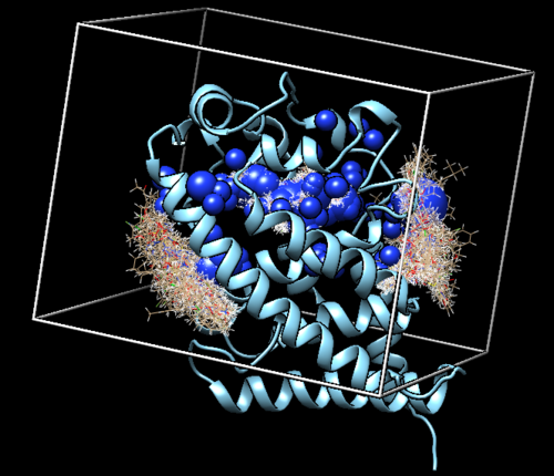
Once opened in Chimera, you will see an image like the one below:
Now we can do some analysis with this Chimera session. To start, we are going to:
Favorites -> Model Panel
In Model Panel we can control the visibility of each of the files that we have loaded in. For now, we are going to uncheck our box, selected spheres and the protein in the Shown category. This will hide those three files to make it easier to visualize. To rank our virtual screen results, we are going to use our ViewDock window. In ViewDock:
Column -> Show -> Grid_Score
Once this panel opens next to the ligands, you can click on the title of the column to organize the ligands from lowest grid score to highest. Selecting one of the ligands will display one of the ligands at a time, and you can push the down arrow on your keyboard to scroll through all of the virtual screen results to visualize them.
We can also visualize the hydrogen bonds that each of the ligands creates with the surrounding residues of the protein. To do this:
Tools -> Structure/Binding Analysis -> FindHBond
In the HBond window we are going to make a few adjustments. First, in the upper right hand box, we are going to make sure that inter-model is checked off. We do not want to find hbonds between residues of the protein or ligands, but between each other. Next, you can choose the HBond color at the top (we use magenta so it is easy to see) and set the line thickness to 4.0. We are going to keep the Relax H-Bond constraints box checked.
Next, we are going to check off the Restrict to Models box. When we do this, we will see a list of all of the models that we currently have loaded into Chimera. For our first HBond analysis, we are going to select all of our virtual screen ligands and the protein. To do this, select the first ligand at the top and hold the shift key to select the rest. Once they are all selected, we are going to go ahead and check off If endpoint atom hidden, show endpoint residue. This will show only the residues of the protein that are making HBonds with the ligand - this makes the visualization in Chimera much less crammed.
Now we can go back to Model Panel and scroll through all of our virtual screen ligands again to view the different HBonds that they make within the binding pocket of the protein. To compare the HBonds that the ligands make to our original ligand, we are going to repeat the HBond analysis process for the ligand. We are going to keep all of the parameters in the HBond window the same as before, except now we are only going to select our dockprepped ligand. We are also going to check off the box Retain currently displayed H-Bonds so we do not lose the HBond data from all of the virtual screen ligands.
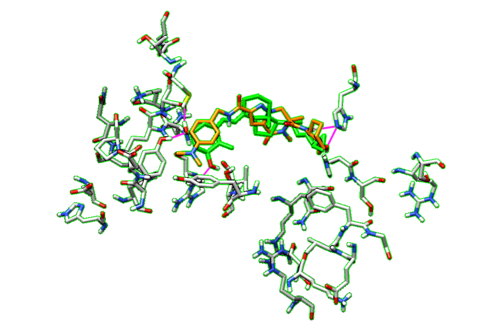
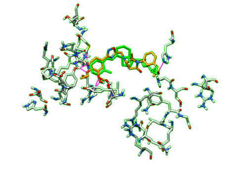
With the dockprepped ligand's HBonds shown now, now we can scroll back through our list of ligands and see how their HBonds compare to our original ligand. Some examples of what this should look like are in the figure below.

